In the Notice of Proposed Rulemaking (NPRM) RIN 1235-A111, DOL proposes to increase and automatically update the salary threshold for exemptions from overtime protections under the The Fair Labor Standards Act (FLSA). I observe in the comments below that DOL understates the economic benefits of the proposed threshold and that the proposed level is consistent with the historical growth in prices and economic output.
In its analysis of the effect of the proposed rule on hours worked, DOL understates the benefits to the workforce by failing to account for employers’ tendency to hire additional workers and to schedule non-overtime work in response to the rule change. Footnote 120 of the NPRM acknowledges that the substitution of overtime hours to non-overtime hours is a possibility, and that DOL understandably “did not have credible evidence to support an estimation of the number of hours transferred to other workers.” Yet it should be noted that this possibility is actually an implication of the fixed-wage model that partially underlies DOL’s analysis.
Ignoring this consequence of the economic model underlying DOL’s analysis causes the NPRM to overestimate the total reduction in economy-wide hours due to the proposed rule, at least in the short run. In particular, when the overtime premia threshold is raised, employers will substitute away from overtime hours and either hire additional workers or schedule additional hours for workers below the 40-hour threshold. Indeed, the fact that there is a spike of 40 hours in the distribution of weekly hours is consistent with the idea that firms substitute away from overtime hours. Moreover, private-sector analyses such as those by the National Retail Federation (2015) and Goldman Sachs (2015) predict increases in employment as employers hire additional workers to work non-overtime hours. This substitution toward non-overtime hours is necessarily implied by the fixed-wage model when output is constant, say in the very short run or in an economy with a large degree of excess capacity. Any offsetting increase in non-overtime hours will be smaller over the medium- to long-term, when both output and capital adjust more easily.
The possibility that some individuals will see increased employment through the extensive or intensive margins has important welfare considerations ignored by the NPRM. Based on empirical evidence describing the extent of overwork in the United States, the NPRM correctly concludes that the proposed rule may improve welfare because it “may result in increased time off for a group of workers who may prefer such an outcome.” At the same time, although many workers in the United States are overworked, a sizable portion of the labor force does not work as many hours as desired (Golden and Gebreselassie 2007; Jacobs and Gerson 2005). Footnote 135 of the NPRM states that the lack of existing scholarly studies precludes quantifying any increase in employment or hours due to the rule, but DOL should make clear that under certain conditions the fixed-wage model underlying their analysis implies that some workers will see an increase in hours. If these workers are under-employed, the shift in the composition of those hours from over-worked to under-worked employees will be a welfare-improving consequence of the proposed rule.
In its calculation of the monetary benefits of reducing hours, the NPRM fails to account for significant externalities associated with high levels of hours worked. The NPRM approximates the benefit an affected worker receives for an hour of additional leisure by the average hourly wage, but this approximation understates the social benefits when the social and private costs of work differ. Some empirical work calculates that longer work hours entail greater energy consumption and consequentially more environmental damage (Rosnick and Weisbrot 2006). And economic theory suggests that long work hours may be detrimental both within and outside of the household (Gersbach and Haller 2005; Folbre, Gornick, Connolly, and Muzni 2013). In a separate section on health benefits of the proposed rule, the NPRM also effectively acknowledges the existence of these externalities cited above, stating that the rule will not only benefit the worker’s welfare through its positive health effects but also “their family’s welfare, and society since fewer resources would need to be spent on health.” Although the NPRM states that its wage-based approximation may overestimate the social benefits of fewer hours worked because not all workers will prefer to reduce their hours, the exclusion of important externalities causes the NPRM to underestimate some benefits of reducing hours.
The NPRM also understates benefits by excluding the possibility that an updated salary threshold will improve pay for hourly workers who are not paid overtime, even when they should be. Rohwedder and Wenger (2015) find that 19 percent of hourly workers are not paid a premium for working overtime hours. While it is unclear if all of these workers are legally required to receive overtime payments (due to occupational exemptions), many of them are not receiving pay promised under the FLSA. The proposed, transparent update to the salary threshold will provide employers an opportunity to revisit whether their employees are paid according to the law.
Finally, the proposed threshold for the overtime weekly salary exemption appears to be consistent with a range of economically appropriate levels. The NPRM proposes raising this threshold to approximately $921, or the 40th percentile of the weekly earnings distribution of salaried employees working full-time. This level is appropriate because it is similar to the exemption threshold that already applied in 1975, after adjusting for inflation ($250 in 1975 dollars, or approximately $1,000 per week in 2014 dollars.). Yet if the labor market’s capacity to bear this regulation is determined by productivity, then this threshold is almost certainly too low. Since 1975, real productivity has grown by more than 72 percent, suggesting an overtime weekly salary threshold of at least $1,720, well exceeding the proposed rule.
Ben Zipperer
Research Economist
Washington Center for Equitable Growth
1333 H St., NW
Washington, DC 20005
References
Folbre, Nancy, Janet Gornick, Helen Connolly, and Teresa Munzi. 2013. “Women’s Employment, Unpaid Work, and Economic Inequality,” in Janet Gornick and Markus Janti, editors, Income Inequality: Economic Disparities and the Middle Class in Affluent Countries, Redwood City CA: Stanford University Press.
Golden, Lonnie and Tesfayi Gebreselassie. 2007. “Overemployment mismatches: the preference for fewer work hours.” Monthly Labor Review. April.
Gersbach, Hans and Hans Haller. 2005. “Beware of Workaholics: Household Preferences and Individual Equilibrium Utility.” IZA Discussion Paper. February. http://ftp.iza.org/dp1502.pdf
Goldman Sachs Global Macro Research. 2015. “The New Federal Overtime Rules: A Greater Effect on Payrolls than Pay.” July 7.
Jacobs, Jerry, and Kathleen Gerson. 2005. The Time Divide: Work, Family, and Gender Inequality. Cambridge MA: Harvard University Press.
Rosnick, David and Mark Weisbrot. 2006. “Are Shorter Hours Good for the Environment? A Comparison of U.S. & European Energy Consumption.” Center for Economic and Policy Research. December. http://www.cepr.net/documents/publications/energy_2006_12.pdf
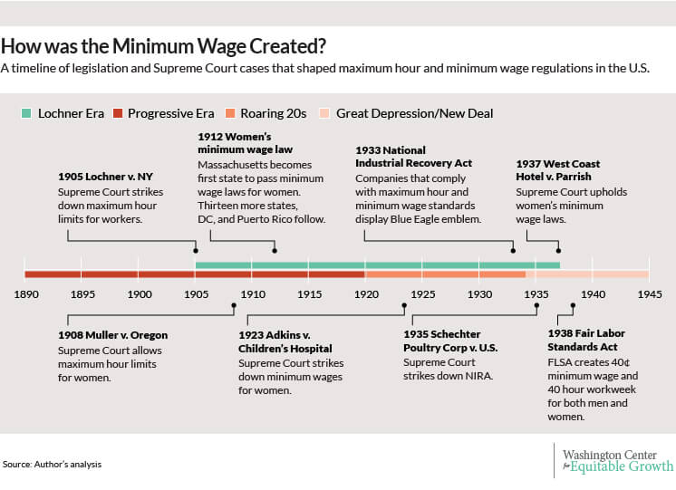
The rapid growth of the “Fight for $15” minimum wage movement and President Barack Obama’s changes to overtime regulations have sparked new rounds of debate over the economic consequences of an increased overtime pay threshold and a higher minimum wage. Advocates of overtime and wage hikes argue these policies protect workers from exploitation and improve job quality. Opponents insist these regulations will hurt workers in the long run, as they will inflict a burden on companies that will be forced to cut jobs. These concerns are nothing new—this debate dates back to the early 20th century, before the minimum wage even existed in the United States and when overtime pay was unheard of.
At the end of the 19th century, economists such as John Bates Clark preached that markets, if left to their own devices, would function at equilibrium levels with the best possible distribution of resources. Rapid industrialization created the Gilded Age of American wealth, and people credited the free market with their increased prosperity.But along with increasing growth, industrialization also sharpened economic inequalities and made certain groups particularly vulnerable to exploitation. Debates over hour and wage limits focused on which groups required labor protections and the best mechanisms for protecting these groups.
Labor regulations began in the 1890s as state-level maximum hour and minimum wage protections, which the U.S. Supreme Court repeatedly struck down. Federal standards were not created until four decades later, when president Franklin Delano Roosevelt and his Secretary of Labor, Frances Perkins, guided the Federal Labor Standards Act into law. (See Figure 1). This issue brief details the arguments that shaped hour and wage limits in the early 20th century.
Figure 1
Women’s maximum hours
U.S. legal historians usually describe the beginning of the 20th century as the “Lochner Era,” a 32-year period characterized by the Supreme Court’s attempt to protect the free market through its constant repeal of labor laws. The Supreme Court actually was discriminatory in its protection of the free market—although it consistently blocked labor laws that applied to men, the high court allowed restrictions on women’s employment. The Supreme Court passed distinct rulings for men and women by emphasizing different doctrines for the two sexes. For men, the court consistently upheld freedom of contract; for women, the court privileged police powers.
The Supreme Court’s gender discrimination began with cases concerning maximum hour limits. In Lochner v New York (1905), the namesake of the Lochner Era, the court justified its decision to strike down the 1895 Bakeshop Act—which placed hour limits on New York bakers—with the freedom of contract doctrine. Freedom of contract comes from the due process clause of the Constitution, which says that no person shall be “deprived of life, liberty, or property without due process of law.” At the time, justices interpreted due process to mean that individuals should be free from restraint except to guarantee the same freedoms to others, and that government could not restrict people’s ability to acquire future property. Limiting the hours that New York bakers worked, proponents argued, took away their liberty to choose the terms of their employment and limited the money they could earn, so maximum hour laws violated freedom of contract.
Just three years later, the Supreme Court set a different standard for women. In Muller v Oregon (1908), it upheld a 1903 Oregon law that prohibited women from working more than 10 hours a day. The court argued that women’s freedom to contract was superseded by the police powers doctrine, which allows government regulation for the purpose of promoting health, safety, morality, and the general welfare of the public. The court found that “as healthy mothers are essential to vigorous offspring, the physical wellbeing of woman is an object of public interest.” In other words, protecting women’s reproductive health was more important than respecting their freedom to contract. Women were also seen as fragile, vulnerable, and lacking the skills necessary to effectively bargain for wages and working conditions, and therefore unable to exercise their freedom of contract. These sex-specific discussions about government-imposed hour limits set the stage for a new conversation: the passage of state minimum wages.
Women’s minimum wages
In 1912, Massachusetts became the first state to pass a minimum wage law that applied only to women and children. Thirteen more states (along with DC and Puerto Rico) followed in the next 11 years.These legislatures passed a patchwork of legislation with a range of wage limits and enforcement mechanisms. States such as Massachusetts created wage commissions to determine industry-specific minimum wages and enforced standards through public shaming, publishing the names of companies that did not comply with the regulations. In contrast, states such as Arkansas set two cross-industry minimum wages for women: experienced women were paid $1.25 a day while inexperienced women only got $1.
The police powers doctrine justified minimum wages for women, but said nothing about how they affected industries. To justify minimum wages on the industry side, academics used the parasitic industries argument. Originally developed by the British economists Beatrice and Sidney Webbs in the late 19th and early 20th centuries, the parasitic industries argument says that businesses who focused on short-term profit maximization instead of long-term efficiency tend to pay workers unlivable wages. Workers receiving these sweatshop wages become a burden to society, since they have to rely on charity or other family members for subsistence. To fix the problem, companies have to either amend their practices to consider the long-term welfare of the company and the workers, or exit the market.
Women’s minimum wage laws grew out of gender norms supporting women’s protection, but at the same time, racial biases led to laws that neglected women of color. Because minimum wage legislation was usually industry-specific, industries such as domestic work, agriculture, retail, and laundry—all dominated by African American workers—were often excluded from regulation. One case in point: The Wage Board in the District of Columbia set a weekly rate for laundry workers that was $1 lower than the across-the-board minimum adequate weekly wage of $16 it has previously chosen. The board explained that since 90 percent of laundry workers were African American, “the lower rate was due to a crystallization by the conference of the popular belief that it cost colored people less to live than white.” By not extending equal minimum wage protections to African American women, minimum wage laws reinforced their lower economic status.
In the next decade, legal changes in women’s status, paired with the economic optimism of the Roaring Twenties, brought a big shift in minimum wage legislation. Ratified in 1920, the 19th Amendment granted Women’s Suffrage. Shortly after, in a victory for more equal gender standards but a loss for labor protections, the Supreme Court issued a ruling that struck down women’s minimum wage laws across the country. In Adkins v Children’s Hospital (1923), the court overturned the 1918 law that created D.C.’s Wage Board, which had set minimum wages for women employed in laundries and food-serving establishments. Reasoning that women were now politically empowered to advocate for themselves in the free market, the Court privileged freedom of contract over police powers and nullified minimum wage laws in the United States.
This optimism about the competitiveness of the free market did not last long. Once the Great Depression hit, people lost faith in the fairness of the U.S. economy. The failure of the banks cultivated distrust of large corporations. People were afraid that business concentration hurt competition and created unfair trusts. The new popular economic narrative of economists such as Joan Robinson and Edward Chamberlain said that imperfect and monopolistic competition dominated the market. This unfair competition gave businesses a huge advantage, which they used to exploit labor. Public opinion shifted toward seeing government intervention not as redistribution but rather as reestablishing a competitive market.
The Fair Labor Standards Act
In this rapidly shifting political and economic climate Franklin D. Roosevelt won the 1932 elections and appointed Frances Perkins as his Secretary of Labor. With decades of experience advocating for labor rights as a social worker and later as Roosevelt’s Secretary of Labor when the future president was governor of New York, Perkins accepted the federal cabinet office on the condition that Roosevelt would commit to supporting her reform platform, which included hour limits and minimum wages for both women and men. Perkins’ platform originally appeared in the National Industrial Recovery Act, which tried to improve working conditions through voluntary industrial participation. Under the proposed law, industries would be able to form alliances, which previously violated anti-trust laws, if they complied with maximum hour and minimum wage standards.In return, participating companies could display a Blue Eagle emblem in their stores, brandishing their patriotism and commitment to post-Great Depression recovery. In Schechter Poultry Corp. v United States (1935), however, the Supreme Court struck down the law, drawing the ire of Roosevelt and forcing Perkins to find a new way to pass labor reform.
Out of growing frustration with the Supreme Court’s challenges to his policies, Roosevelt came up with a plan to pack the court. He set off a campaign to reform the Supreme Court so he could appoint additional members to the court who would vote in line with his New Deal reforms. Faced with this existential threat and greater public support for labor laws, in 1937 the Supreme Court ruled in favor of Washington state’s minimum wage law for women in West Coast Hotel Co. v Parrish. The court’s ruling de-emphasized the freedom of contract, reversing its 1923 decision and opening the door for future minimum wage legislation.
Following the Supreme Court decision, Perkins and Roosevelt sent a maximum hour and minimum wage bill to Congress. The original draft of the bill had called for industry-specific, regionally variant minimum wages to account for regional differences in prices and cost of living. As the bill made its way through Congress, two more opposition groups emerged: unions and northern industries. Unions feared that government-imposed wage and hour restrictions would undermine their influence in collective bargaining. Northern industries opposed regionally specific wages for fear that industries would follow the cheap labor south. To appease these two groups, Roosevelt and his Democratic allies in Congress tweaked the bill to make it more popular. Roosevelt appeased the unionists’ fears in his State of the Union address by emphasizing that more desirable wages should continue to be the responsibility of collective bargaining. Lawmakers suggested a national minimum wage to satisfy northerners, but set the wage low enough to appease southerners.
In its final form, the Fair Labor Standards Act of 1938 mandated a 44-hour workweek, scheduled to decrease to 40 hours in three years, with time-and-a-half overtime wages. The new law also created a minimum wage of 25 cents an hour, set to increase by 5 cents a year to reach 40 cents an hour by 1945. The original law was not universal. It included exemptions for agricultural, domestic, and some union-covered industries—once again, mostly industries dominated by African Americans.Since the law lacked a mechanism for automatically increasing wages beyond 1945, it has been updated over the decades to increase wages and broaden industry (and racial) coverage. In the most recent revision to the Fair Labor Standards Act in 2009, the federal minimum wage was increased to $7.25 an hour.
Conclusion
The intellectual history of maximum hours and minimum wages is a story of debates over which groups should be protected from exploitation and what form this protection should take. Concerns over women’s health, ambivalence toward African American rights, and advocating for unorganized workers dominated the debate at different points. As social views changed, so did economic policies. Today, women account for two-thirds of minimum wage earners and people of color account for two-fifths.Studying the history of the minimum wage should compel policymakers to question how social priorities influence different groups, who is considered worthy of protection, and to what extent their welfare is considered. By implementing effective maximum hour and minimum wage regulations, policymakers can protect vulnerable workers’ standard of living to encourage productivity, push companies to increase their efficiency, and consequently cultivate long-term equitable growth.
-Oya Aktas is a Summer 2015 intern for the Washington Center for Equitable Growth
A snapshot of the long-term impacts of universal prekindergarten
If the United States were to invest in a public, voluntary, high-quality universal prekindergarten program starting in 2016, what would its impacts be over time? Toggle between the buttons to visualize the different impacts of universal prekindergarten programs across the U.S. or click on a state to learn more about the program in that state.
This study looks to quantify the long-term benefits and costs of investing in a high-quality universal prekindergarten available to all three- and four-year olds across the United States. But before delving into the report, use the interactives below to explore how a universal prekindergarten would affect the nation or even your state.
Who would participate?
Currently, across the United States, only 17 percent of three- and four-year-olds (1,336,695 children) participate in state-sponsored prekindergarten, and another 38 percent attend Head Start or private preschool. Unfortunately, the quality of these programs varies significantly across and even within states, which means that preschoolers do not always experience the same benefits or long-term effects. If a universal program were enacted and fully phased in by 2017, 86 percent of three- and four-year-olds (6,960,916 children) would be enrolled in prekindergarten, benefiting from a high-quality early childhood education.
What are the benefits?
Research has established that high-quality prekindergarten education can generate significant long-run benefits for program participants, their families, and even other non-participants. For example, longitudinal studies have shown that, aside from improved educational achievement, children who have attended a prekindergarten program have spent less time in special education and had lower grade retention rates. Program participants also experience less child maltreatment and reduced crime, smoking, and depression rates. In addition, both participants and their parents have higher projected earnings, which subsequently increases government tax revenue.
If a universal prekindergarten program were to start in 2016, by 2050, there would be over $304 billion in total benefits for the U.S. In 2050, that amounts to savings of $748.51 per capita. How do these total benefits break down? $200.41 per person is attributed to savings to government, $281.81 per person comes from increased compensation, and $266.27 is accounted for by savings to each individual from better health and less crime.
What are the costs?
Currently, the U.S. spends an average of $45 per capita per year on preschool programs, special education services, and Head Start. In 2017, when a universal prekindergarten program is fully phased in, it would take an investment of $79 more per capita per year to maintain a high-quality prekindergarten program.
There are three main costs associated with a high-quality universal prekindergarten program: the cost of the program, increased high school attendance, and increased college attendance. The program itself is based on Chicago’s comprehensive high-quality Child Parent Center half day program, and thus, the costs take into account the multitude of services that are provided at the Child Parent Center offset by the current spending on similar early childhood education programs as to not double count expenditures. Because studies have shown that students who attend prekindergarten have higher high school completion rates and are more likely to attend college, these usage costs are also factored into the total cost of a universal prekindergarten program.
In 2050, these costs add up to $35 billion, or $84.54 per capita. $74.27 per capita is attributed to program costs, $2.35 comes from increased high school usage per person, and the remaining $7.92 per person is accounted for by increased college attendance.
How do the benefits compare to the costs?
If a high-quality universal prekindergarten program were to start in 2016 and be fully phased in by the end of 2017, the program would require $26 billion in additional taxpayer dollars. Over time, the cost would eventually grow to include the cost of additional high school and college usage. But in just 8 years, by 2024, the benefits of the program would outstrip the costs. By 2050, there would be more than $304 billion in total benefits compared to merely $35 billion in total costs, yielding net benefits of $270 billion. By 2050, for every dollar invested in a universal program, there would be $8.9 in returns.
Last year, our colleague Elisabeth Jacobs referred to the fate of young people in today’s slack labor market as “a cruel game of musical chairs” because there aren’t enough jobs to employ everyone at their full earning potential. Workers with college degrees tend to win out in the competition for the few jobs that are available, but many must settle for lower-paying jobs than similarly credentialed workers entering the workforce in previous decades. Those without college degrees, in turn, are driven into even lower paying work or pushed out of the labor market entirely. Economists refer to this phenomenon as “filtering-down,” with the best-educated workers increasingly filling jobs lower and lower on the job ladder.
The dire experience of these workers with college degrees displacing workers with less formal education stands in strong contrast to the widely–heldview in economic and policymaking circles that the main problem facing the U.S. economy is a shortage of highly-educated workers. If college-educated workers were in short supply, then we would expect their wages to rise as employers attempted to lure them away from their competitors. Yet the inflation-adjusted value of the wages of college-educated workers has barely increased in the 21st century.
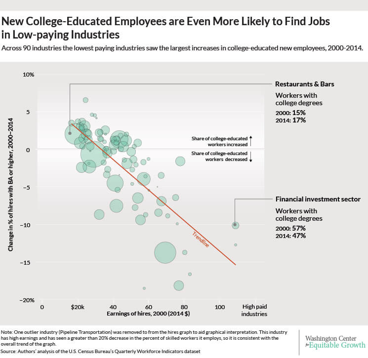
What’s more, between 2000 and 2014 (the last year for which complete data are available), the employment of college-educated workers has increased much more rapidly in low-earning industries than in high-earnings ones. If there weren’t enough college graduates to go around, then the opposite should be happening because high-earnings industries would presumably be outcompeting low-earnings industries to hire college-educated workers. Our new analysis of the data from the U.S. Census Bureau’s Quarterly Workforce Indicators strongly suggests that college-educated workers are more likely to “filter down” the job ladder than to climb it.
The QWI dataset is a comprehensive administrative source for information on flows in and out of employment, collecting information on total employment, hires, “separations” (workers either quitting their jobs, getting laid off, or fired for cause), and earnings. The data are disaggregated along many dimensions, including workers’ education level and the industries where they work. We can, for example, look at the share of employees in restaurants and bars that have a Bachelor’s degree or more, or the share of workers on Wall Street who have less than a high school degree.
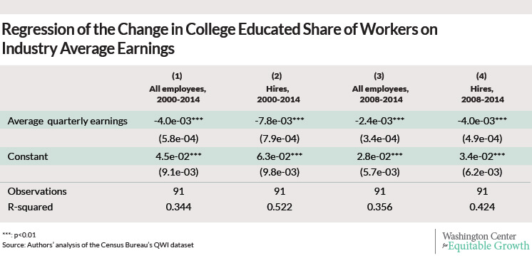
Our analysis examines the average earnings of workers in the 91 industry groups—identified by their 3-digit coding in the North American Industrial Classification System–which together account for nearly all employment in the United States, alongside the share of workers in each industry with a college degree or more. While not definitive, the most striking finding is that the industries with the lowest earnings for all employees are experiencing the largest increases in the share of workers with a college education or higher. Our analysis, for example, finds that 16.3 percent of all workers who work in restaurants and bars in the United States have attained a Bachelor’s degree or more, compared to 14.2 percent in 2000. In contrast, high-paying industries such as the financial sector saw their share of college-educated workers decrease, from 65.2 percent in 2000 to 56.1 percent in 2014 (See Figure 1).
Figure 1
This “filtering down” trend in the employment of college-educated workers is even more acute when we look at recent hires rather than overall employment. The trend line over 2000-2014 is even more steeply downward sloping for hires than for all employees, highlighting the cruel game of musical chairs. In short, a college degree is becoming increasingly less predictive of employment in a high-earnings industry. (See Figure 2.)
Figure 2
If instead of plotting the change in employment of college-educated workers or the change in recent hires of college-educated workers on the vertical axis—as we have done in Figures 1 and 2—we had alternatively plotted the share of college-educated workers in total employment, or the share of college-educated workers in recent hires, then we would see that industries with higher average earnings tend to employ more credentialed workers. In other words, the trend line we would see in the alternative charts would slope up, not down. Findings of that kind, which depict the higher average earnings of college-educated workers, are typicallytrumpeted as evidence that the only thing preventing young, under-employed workers from finding a good job is their lack of a Bachelor’s degree. But what our analysis demonstrates is that this relationship has gotten less positive since 2000. (See the data appendix below for a complete description of the data and our methodology.)
This means that the changing share of workers with a college degree or more across industries is unlikely to be due to “skill-biased technical change” in low-earnings industries, since by and large workers in those industries are less prone to technological substitution. Think bartenders and busboys. Those workers perform what economists call “non-routine, manual” tasks that can’t easily be performed by pre-programmable machines. Nor does the rise in the share of college-educated workers in lower-paying industries merely reflect that there were fewer such workers in these industries prior to 2000, because the same trend is true among recent hires as among employees overall.
Finally, the increased hiring of workers with college degrees has not boosted the relative pay in those low-paying industries. The patterns are quite similar whether we calculate industry average earnings in 2000 or in 2014 because average earnings across industries haven’t changed very much. What’s changed is the education mix of workers.
The implication of all of these findings is that the U.S. labor market doesn’t lack for college-educated workers. Workers who have degrees are already taking jobs further and further down the job ladder. Encouraging or subsidizing higher education attainment will not solve the fundamental problem facing workers in the current job market: There are not enough jobs.
Data appendix
The U.S. Census Bureau’s Quarterly Workforce Indicators is a comprehensive administrative dataset of employment “matches,” meaning labor market relationships between employers and employees. The existence of a match (employment), the beginning of a match (hires), and the end of a match (separations) are observed in a given quarter, along with average earnings of workers in each group of hired workers, employed workers, and separated workers. The QWI is disaggregated by geography, industry, and many demographic characteristics, including, for our purposes, education attainment (discussed more completely below).
There are two predominant underlying sources of the QWI data: U.S. Census data and state unemployment insurance filings by businesses. QWI is the publically available version of a dataset called Longitudinal Employer-Household Dynamics, or LEHD, which follows individual workers from job to job over the course of their careers. QWI, however, does not track individual workers over time. Instead, quarter-by-quarter, it counts up all the flows described in the previous paragraph, for each detailed sub-population and employer category.
Because state-provided data from the unemployment-insurance system are critical to constructing LEHD and hence the QWI, and because states only began to participate in the LEHD at different points in time, the data are available as an unbalanced geographic panel. Every state except Massachusetts is currently providing data to the program, but the start dates vary by state. Enough states have joined by about 2000 that the literature has labeled QWI nationally representative from that point forward, which covers all the data reported in this exercise. We aggregate the data across states to create our industry-education disaggregation.
LEHD does not actually observe the education levels of most workers. For those it does not observe, education is imputed from other worker characteristics using Census Bureau microdata (mostly from the 2000 Decennial Census). That is the most likely reason why the QWI-reported share of college-educated workers has decreased by slightly more than one percentage point overall, and by substantially more in some industries. The imputation procedure works best around the date when its source data was collected (2000), and increasingly less well as we get further away from that date. The Current Population Survey, a representative sample of the population collected continuously, reports that the overall share of college-educated workers in the economy increased by approximately five percentage points between 2003 and 2012, and has only declined by a small amount in a very few industries.
The education imputation in QWI complicates the inference from exercises such as the one we present here, because the whole point of our interpretation is that educational attainment has become less predictive of workers’ experience in the labor market, and in particular, of their earnings, as better-educated workers are forced to take worse jobs. The effect of the data imputation, however, is most likely to mute the phenomena we highlight: if credentialed workers are taking jobs further down the labor market hierarchy, then workers who take jobs further down the hierarchy than they did in the past would be more likely to be misidentified as lacking educational qualifications. For that reason, we believe the imputation of education data means that our results understate the effect of filtering-down.
Tentative confirmation for this can be found in a regression of the change in the share of young workers on industry average earnings, which yields an even-more-sharply negative slope than Figures 1 and 2. In other words, young workers are filtering down the labor market even more starkly than BA-educated ones, according to QWI. Since young workers are more likely to have college degrees than retirees, the education-based regressions we present here probably understate the cruelty of the cruel game of musical chairs.
In order to construct Figures 1 and 2, we use a NAICS 3-digit Industrial Sector disaggregation of the QWI’s 2015Q3 Sex by Education files with all firm size and age categories for all available states and the District of Columbia. The data are smoothed using a four-quarter moving average, and nominal earnings are adjusted for inflation (to 2014 dollars) using the Consumer Price Index for all Urban Consumers, or CPI-U. We use the “stable jobs” concept, meaning only “full-quarter employment” is counted. A worker is “full-quarter employed” at a given match if and only if that worker has positive earnings from that match in the quarter itself and (at least) the ones preceding and subsequent. (Similarly, a “full-quarter hire” is one in which positive earnings are observed in the preceding, current, and subsequent quarters but not two-quarters-ago.)
The dependent variables in the regression are calculated from either EmpS or HiraS (for employment and hires respectively), and the dependent variables are correspondingly EarnS or EarnHiraS. We use the education category corresponding to a “BA or more” to calculate college-educated shares of employment and hires, and we exclude workers aged 24 or under since QWI does not report education attainment for that age group. (See Figure 3.)
Figure 3
The raw data and the Python script we used to clean and reshape the raw data are available at Equitable Growth’s GitHub.
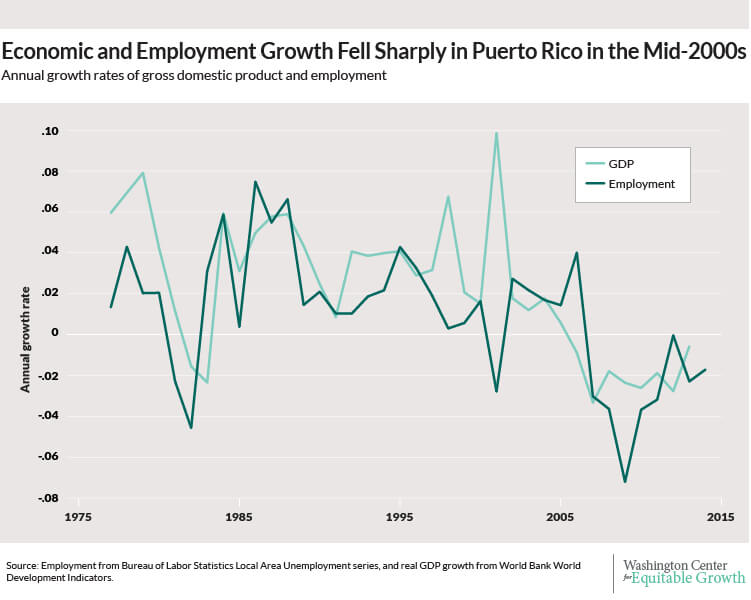
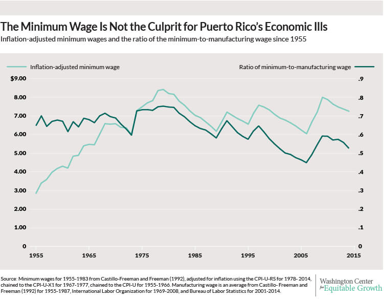
Puerto Rico today faces a serious debt crisis, recently defaulting on a bond payment. The proximate cause is a slowdown in economic growth since the mid-2000s, which has reduced tax revenues, and a declining labor market, where employment growth has been mostly in the red since 2007.
Figure 1
There are many explanations for the economic downturn and the resulting fiscal crisis, but some commentators have incorrectly blamed the island’s high minimum wage. To be sure, the federal minimum wage—which has applied to Puerto Rico since 1983—is much more binding there than it is on the mainland. Because hourly wages are substantially lower in Puerto Rico compared to the U.S. mainland, the federal minimum wage policy affects more of the workforce there. In 2014, for example, the federal minimum wage stood at 77 percent of the median hourly wage in Puerto Rico, compared to 42 percent in the United States. For comparability with existing estimates, if we consider wages of full time workers only, these figures are approximately 70 percent in Puerto Rico and 38 percent in the United States, respectively. Finally, the minimum wage stands at 56 percent of the wage earned by production workers in manufacturing, compared to 38 percent in the United States. Clearly, the Puerto Rico’s minimum wage exceeds the cautious rule-of-thumb of 50 percent of median wage of full-time workers suggested by one of us in previous work.
But does that make it a probable culprit for the island’s current debt and economic troubles? The short answer is: not very likely. The major problem with a minimum wage-centric explanation is timing. There has been no change in the relative minimum wage between Puerto Rico and the mainland over the past 32 years. And since the federal standard has not kept up with wage growth on the island, the bite of the minimum wage in Puerto Rico has eroded over this period.
First, the current inflation-adjusted value of the federal minimum wage is not higher than it was when Puerto Rico first adopted it. Puerto Rico’s minimum wage is worth slightly less today than in 1983, even though its economy, in terms of GDP per capita, has grown by 72 percent.
Second, real wages in Puerto Rico were lower three decades ago. As a result, if we measure the bite of the minimum wage as the ratio of the minimum wage to the average manufacturing wage, the bite was closer to 70 percent when Puerto Rico first adopted the federal minimum wage, much higher than it is today, at 53 percent. (We use the manufacturing wage for this comparison because the median wage series is not available over as long a historical period, to the best of our knowledge.)
Figure 2
Additional evidence suggests the current minimum wage in Puerto Rico is also less consequential today than it was during the 1980s. In 1983 the share of Puerto Rico’s workers affected by the minimum wage was around 44 percent, but by 2010 this share had fallen to around a third. It is difficult to explain the economic crisis in Puerto Rico starting in the mid-2000s with a minimum wage that is, if anything, on the wane.
Finally, we should note that some recent reports have also incorrectly measured the level of the minimum wage in Puerto Rico, stating that a full-time minimum wage worker in Puerto Rico earns 77 percent of the nation’s per capita income, as opposed to 28 percent in the United States. Data from the World Bank suggests that although the ratio of 28 percent is correct for the mainland, the statistic for Puerto Rico is closer to 53 percent as of 2013, the last year in which complete data are available.
Does this mean the island’s minimum wage has no negative consequences? It’s possible that the minimum wage led to somewhat lower levels of employment than would otherwise occur. After all, the minimum wage is much higher in Puerto Rico than the kind of increases we have studied elsewhere in the United States, where we find employment effects that are small and oftenindistinguishablefromzero.
But clear evidence of job losses due to Puerto Rico’s relatively high minimum wage remains elusive. The two main scholarly papers on the topic reach different conclusions when analyzing the original Puerto Rican introduction of the federal minimum wage in 1983. In their 1992 paper, “When the Minimum Wage Really Bites: The Effect of the U.S. Level Minimum on Puerto Rico,” economists Alida Castillo-Freeman at the National Bureau of Economic Research and Richard Freeman at Harvard University found evidence of moderate-sized job losses by comparing unemployment trends over time, and by comparing wages and employment across industries on the island.
Yet in a careful reanalysis of the same data in 1994, Princeton University economist Alan Krueger found that some of the findings by Castillo-Freeman and Freeman proved fragile. One case in point: the more negative estimates from cross-industry comparisons were in part driven by the over-representation of many narrow manufacturing industries in their sample. And there was some indication of the effects occurring, implausibly, prior to the actual increases in the minimum wage. Finally, while some of the episodes of minimum-wage increases on the island were associated with higher unemployment, the opposite was true during other episodes.
Control groups for the Puerto Rican case are not easy to find, and so it is difficult to decipher what would have happened if the minimum wage in Puerto Rico were much lower. But, while there may be disagreement on whether the Puerto Rico’s minimum wage has caused the unemployment rate to be somewhat higher, both Professors Freeman and Krueger are in complete agreement today that it is unlikely either to be a major factor behind the current economic crisis, or an important part of the solution.
Indeed, the long-run decline in the bite of the minimum wage presents a serious challenge for those arguing otherwise, since the timing of the crisis is inconsistent with minimum wage having played a real role in it. Reasonable people may differ on the costs and benefits of applying the federal minimum wage to Puerto Rico. But it would be misguided to expect minimum wage policy to provide a cure for the island’s ailments.
—Arindrajit Dube is an associate professor of economics at the University of Massachuetts-Amherst. Ben Zipperer is an economist at the Washington Center for Equitable Growth.
Recently available research looks across developing and advanced countries and within the United States to examine the effects of economic inequality on economic growth, well-being, and stability.
Research is beginning to find that economic inequality harms economic growth over the long term and that countries with less income and wealth disparities and a larger middle class boast stronger and more stable economic growth. Yes some studies also suggest that in the short run, greater economic inequality may spur growth before hindering it over the longer term. Overall, however, there is growing evidence that more equitable societies are associated with higher rates of long-run growth.
Evidence from across states within the United States
Studies that look at the relationship between inequality and growth in the United States mirror those of international studies—less inequality is associated with long-term growth and is particularly associated with lower income growth for those at the top of the income ladder. But the international results also indicate that in the short run economic growth may not be harmed by inequality even in the United States. Here are some key findings:
Ugo Panizza of the U.N. Conference on Trade and Development finds a negative relationship between inequality and growth across U.S. states. A larger share of income accruing to the middle class is associated with higher growth rates, while higher inequality leads to lower growth rates.[i]
Using data for 48 states from 1960 to 2000, Mark Partridge of Ohio State University finds that in the short run inequality is positively related to growth while in the long run the income share of the middle class is positively associated with more robust growth.[ii]
Economists Mark Frank and Donald Freeman of Sam Houston State University, using methods focusing on longer run trends, find a strong, negative relationship between inequality and growth.[iii] Though, Mark Frank released a subsequent study using new state-level inequality and growth data from 1945 to 2004 that found higher income concentration increased short-run growth. This second paper by Frank highlights some of the nuances of the relationship between inequality and growth.[iv]
In a recent book, “Just Growth: Inclusion and Prosperity in America’s Metropolitan Regions,” Chris Benner, associate professor of community and regional development at University of California-Davis, and Manuel Pastor, professor of American studies and ethnicity at University of Southern California, show that less economic inequality within regional economies is linked to regional prosperity.[v]
In a 2014 paper by Roy van der Weide of the World Bank and Branko Milanovic of the City University of New York looks at income growth instead of gross domestic product for inequality measures at different points along the income distribution, using state-level data in the United States. They find that high levels of economic inequality decrease income growth for those at the bottom of the income distribution.[vi]
Milanovic and van der Weide also find that high levels of inequality at the bottom of the income ladder is associated with slightly faster income growth at the top of the ladder.[vii]
Milanovic and van der Weide’s research is consistent with earlier work by then University of Massachusetts-Amherst economist Jeffrey Thompson (now at the Federal Reserve Board in Washington, DC) and Congressional Budget Office analyst Elias Leight, who look at the effects of inequality on incomes across households. They found that increases in the incomes of those at the top of the income ladder, measured by either the top 10 or 1 percent, are associated with declines in incomes of low and middle-income households.[viii]
International comparisons
In the most recent literature of international comparisons, a new, somewhat nuanced theme is emerging that high inequality is bad for economic growth over long time horizons and that high inequality is particularly bad for those on the bottom of the income spectrum. But in the short run, most of the research agrees that high inequality can be associated with faster economic growth, but the benefits tend to flow to the top for that short period of time. Some of the key findings in this research arena include:
In May 2015, the Organisation for Economic Co-operation and Development (comprised of developed and leading developing nations) issued its most recent findings in its report “In it together: Why Less Inequality Benefits Us All.” The OECD found that between 1990 and 2010, gross domestic product per person in 19 core OECD countries grew by a total of 28 percent, but would have grown by 33 percent over the same period if inequality had not increased after 1985. The report concludes that “income inequality has a sizeable and statistically significantnegative impact on growth.”[i]
To better understand the time dimension of these trends, International Monetary Fund economists Andrew G. Berg and Jonathan D. Ostry looked at periods of growth instead of duration. They find that “countries with more equal income distributions tend to have significantly longer growth spells.” They also found that inequality was a stronger determinant of the quality of economic growth than many other commonly studied factors such as external demand and price shocks, the initial income of the country (did it start out wealthy or very poor?), the institutional makeup of the country, its openness to trade, and its macroeconomic stability.[ii]
In a 2014 extension of this work, Ostry, Berg, and their IMF colleague Charalambos Tsangarides include an analysis of the impacts of income redistribution to ameliorate income inequality as well as market inequality. They find that economic growth is lower and periods of growth are shorter in countries that have high inequality as measured by the Gini coefficient of income after taxes and transfer. (The Gini Coefficient is a common measure of income inequality.) In the same paper, the researchers show that transfers (redistributions of income from upper to lower income individuals) do not harm economic growth—at least up to a point consistent with policies in other wealthy nations.[iii]
Diego Grijalva of the University of California-Irvine finds that some economic inequality (not extreme inequality though) may have some positive short- and medium-term effects on economic growth, but in the long run high levels of economic inequality tend to be detrimental to economic growth.[iv]
Daniel Halter and Josef Zweimuller of the University of Zurich, and Manuel Oechslin of the University of Bern find that there are methodological differences in the papers that find positive relationship between inequality and growth and those that find a negative relationship. Specifically, those papers that examine inequality’s effect on growth over time within countries tend to find a positive relationship but those that use cross-sectional comparisons find a negative relationship. They posit that the time-difference methods are detecting short-term positive effects to growth, while the cross-sectional methods pick up the long-term negative effects for growth when there is persistently high or growing inequality. [v]
In 2011, Dan Andrews of the OECD, Christopher Jencks at Harvard University, and Andrew Leigh at Australian National University looked at inequality in the form of concentration of income at the top of the income spectrum (primarily the top 10 percent, but they also tested the top one percent). The results were somewhat contradictory, leading them to conclude that “inequality at the top of the distribution either benefits or harms everyone and therefore depends on long-term effects that we cannot estimate very precisely even with these data.”[vi]
Conclusion
Economic theory supports conflicting narratives about the potential impact of economic inequality on economic growth. There are some ways that inequality could boost growth and other ways that it could retard growth. Furthermore, there are numerous possible mechanisms that could relate inequality to growth and many of these channels would have conflicting outcomes. Because theory cannot provide strong guidance, it is imperative to use data and analysis to understand the relationships.
Studies that look at the longer-term growth implications of economic inequality find that inequality adversely affects growth rates and the duration of periods of growth, while those that focus on short-term growth find that inequality is not harmful and may be associated with faster growth. Furthermore, studies that look at the impact of inequality on different levels of the income distribution find that inequality is particularly bad for the income growth of those not at the top.
Research on inequality and growth may be approaching a new consensus on the general implications of inequality on economic growth, but more work is needed to fully understand the specifics of how inequality affects growth. In particular, now that the United States is approaching a level of inequality that is very rare among developed economies and more closely resembles a developing economy, which mechanisms apply? These are questions that will require continued updates to the data and methods.
[i] OECD, In It Together: Why Less Inequality Benefits All (Paris: OECD Publishing, 2015).
[ii] Andrew Berg and Jonathan Ostry, Inequality and Unsustainable Growth (Washington, DC: International Monetary Fund, 2011).
[iii] Jonathan D. Ostry, Andrew Berg, and Charalambos G. Tsangarides, Redistribution, Inequality, and Growth, Discussion Note, IMF Staff Discussion Note (Washington, D.C.: International Monetary Fund, February 2014), http://www.imf.org/external/pubs/ft/sdn/2014/ sdn1402.pdf.
[iv] Diego F. Grijalva, Inequality and Economic Growth: Bridging the Short-Run and the Long-Run, November 29, 2011, http://escholarship.org/uc/item/4kf1t5pb.
[v] Daniel Halter, Manuel Oechslin, and Josef Zweimüller, “Inequality and Growth: The Neglected Time Dimension,” Journal of Economic Growth 19, no. 1 (March 1, 2014): 81–104, doi:10.1007/s10887-013-9099-8.
[vi] Dan Andrews, Christopher Jencks, and Andrew Leigh, “Do Rising Top Incomes Lift All Boats?,” The BE Journal of Economic Analysis & Policy 11, no. 1 (2011), http:// www.degruyter.com/view/j/bejeap.2011.11.issue-1/ bejeap.2011.11.1.2617/bejeap.2011.11.1.2617.xml.
[i] Ugo Panizza, “Income Inequality and Economic Growth: Evidence from American Data,” Journal of Economic Growth 7, no. 1 (2002): 25–41.
[ii] Mark Partridge, “Does Income Distribution Affect U.S. State Economic Growth,” Journal of Regional Science 45 (2005): 363–94.
[iii] Mark W. Frank and Donald Freeman, “Relationship of Inequality to Economic Growth: Evidence from U.S. StateLevel Data,” Pennsylvania Economic Review 11 (2002): 24–36.
[iv] Mark W. Frank, “Inequality and Growth in the United States: Evidence from a New State-Level Panel of Income and Inequality Measures.” Economic Inquiry 47, no. 1 (January 2009): 55–68.
[v] Chris Benner and Manuel Pastor, Just Growth: Inclusion and Prosperity in America’s Metropolitan Regions (New York: Routledge, 2012).
[vi] Van der Weide, Roy, and Branko Milanovic. “Inequality Is Bad for Growth of the Poor (But Not for That of the Rich).” World Bank Policy Research Working Paper 6963 (July 2014). http://www-wds.worldbank.org/servlet/ WDSContentServer/WDSP/IB/2014/07/02/000158349_2 0140702092235/Rendered/PDF/WPS6963.pdf.
[viii] Jeffrey Thompson and Elias Leight, Searching for the Supposed Benefits of Higher Inequality: Impacts of Rising Top Shares on the Standard of Living of Low and MiddleIncome Families (Amherst: Political Economy Research Institute – University of Massachusetts, Amherst, 2011), http://www.peri.umass.edu/fileadmin/pdf/working_papers/working_papers_251-30.
Elisabeth Jacobs, Senior Director for Policy and Academic Programs, Washington Center for Equitable Growth, testifying before the United States Joint Economic Committee on “What Lower Labor Force Participation Rates Tell Us about Work Opportunities and Incentives”
I would like to thank Chairman Coats, Ranking Member Maloney, and the rest of the Committee for inviting me here today to testify.
My name is Elisabeth Jacobs and I am Senior Director for Policy and Academic Programs at the Washington Center for Equitable Growth. The center is a research and grant-making organization dedicated to understanding what grows our economy, with an emphasis on understanding whether and how economic inequality impacts economic growth and stability.
I am pleased to be here today to address an important topic for understanding the health of the labor market and the economy overall: the labor force participation rate, which currently stands at 62.6 percent. The continued decline of the unemployment rate since 2010 is the most commonly cited piece of evidence that the labor market is recovering. Indeed, it is undeniable that the labor market has improved considerably in the years since the Great Recession, as unemployment has fallen to 5.3 percent, its lowest rate in seven years. Despite this progress, however, the labor market remains troubled. Simply relying on the unemployment rate as an indicator of the health of the job market masks underlying problems, many of which have persisted for decades. In order to fully understand the current state of the labor market, policymakers need to take into account not just the unemployment rate, but also other indicators of how the labor market is functioning, including the labor force participation rate.
My testimony draws five major conclusions:
The labor market is recovering from the deepest economic downturn since the Great Depression. The private sector has added 12.8 million private-sector jobs over 64 straight months of job growth, the longest streak of private-sector job creation on record. The unemployment rate is down to 5.3 percent, a seven-year low.
While the labor market is on the mend, looking solely at the falling unemployment rate overstates that recovery. Other indicators of labor market health, including the labor force participation rate, suggest that there is more work to be done.
The decline in the labor force participation rate predates the Great Recession and is mainly the result of several structural changes in the labor market, including the aging of the workforce.
Recent declines in the labor force participation rate that are not explained by long-standing structural changes are largely due to persistent business cycle effects. Five years into the labor market’s recovery from the most severe recession in recent history, demand remains slack.
Policy can play an important role in boosting the labor force participation rate, but policymakers need to focus on the correct levers. Persistent slack demand suggests that fiscal and monetary policies are an important first step. In the absence of political action on those fronts, however, family-friendly policies and criminal justice reform are important options.
The rest of my testimony will 1) discuss recent trends in the unemployment rate and other measures of the health of the labor market, 2) examine the potential reasons for the long-run decline in the labor force participation rate, and 3) review the research on the trends in the labor force participation rate since the Great Recession. I conclude by suggesting key implications for policy moving forward.
Trends in the unemployment rate and the health of the labor market
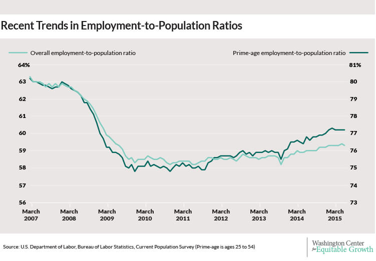
The Great Recession’s impact on the labor market was devastating. In December 2007, the month the recession began according to the National Bureau of Economic Research, the unemployment rate was 5 percent. By the end of the recession, in June 2009, the unemployment rate hit 9.5 percent and continued to climb until it peaked at 10 percent in October 2009. Over the past five and a half years, the labor market has made substantial progress back toward where it was before the financial crisis. The economy is in the midst of the longest streak of private-sector job growth on record, with 12.8 million jobs created over 64 straight months. The most notable headline has been the continued downward trajectory in the unemployment rate. Joblessness as defined by the official unemployment rate has been on the decline more than 5 years, and stood at 5.3 percent in June, according to the latest data from the Bureau of Labor Statistics. Indeed, an observer looking solely at the unemployment rate might conclude that the labor market is roughly as healthy as it was prior to the Great Recession. (See Figure 1.)
Figure 1
Yet, other measures of the labor market tell a more complicated story. Consider the employment-to-population ratio, which is the share of the total population currently employed. Whereas a decreasing unemployment rate is a sign of improvement in the labor market, an increasing employment ratio can be an even stronger signal of improvement. Unfortunately, the trend in the employment ratio is less sanguine than trend in the unemployment rate.
The employment ratio plummeted during the Great Recession, unsurprisingly. In December 2007, the employment ratio was 62.7 percent, and it fell to a nadir of 58.2 percent in November 2010. The share of the population currently employed has improved over the course of the recovery, and has been growing for just under four years, reaching 59.3 percent in June. Yet it remains 3.4 percentage points below its level prior to the Great Recession, suggesting continued weakness in the labor market. A second key point to keep in mind is that, like many indicators of underlying labor market health, the downward trajectory of the employment ratio pre-dates the Great Recession. The employment ratio peaked in December 2006, a year before the financial crisis, and was higher still in April 2000, when it hit 64.7 percent.
The prime-age employment ratio, or the share of the total population between the ages of 25 and 54 years old with a job, has followed a similar trajectory. Its pre-recession peak, in December 2007, was 79.7 percent. But the prime-age employment ratio was just 77.2 percent in June, a current gap of 2.5 percentage points. The labor market has made considerable gains in the light of the worst recession since the Great Depression. But looking at these employment-to-population ratios is one indication that reveals how those gains are incomplete. (See Figure 2.)
Figure 2
Why does the unemployment rate indicate a more complete labor market recovery than does the employment rate? The answer has to do with the intertwined and complicated relationship between the unemployment rate and the labor force participation rate.
The unemployment rate is calculated by the Bureau of Labor Statistics using the Current Population Survey, or CPS, a survey that interviews a sample of households every month and details information about individuals over the age of 16. Individuals who had a job during the week they were interviewed are counted as employed. But not all workers who lack a job are counted as unemployed. According to the CPS, a worker is only officially unemployed if she lacks a job, has actively searched for a job in the last four weeks, and is available to work. Employed workers and officially unemployed workers are together the “labor force.” Any worker without a job who is not counted as officially unemployed is considered to be “not in the labor force.” The official unemployment rate is then calculated by dividing the number of officially unemployed by the labor force. It is an important measure of labor market health because of the clarity of what’s being counted: the unemployment rate is a clear indication of the share of Americans who are actively looking for work. The labor force participation rate is the labor force divided by the total population.
When we think about the unemployment rate declining, we usually think of a situation where an unemployed worker gets a job, moving from unemployment to employment. The ranks of the unemployed would decline, while the size of the labor force would stay the same. The result would be a lower unemployment rate. But the unemployment rate could decline in another way. An unemployed worker could drop out of the labor force, reducing the size of both the number of officially unemployed workers and the labor force. This also would also lead to a decline in the unemployment rate.
An example can help clarify this point. Imagine a labor market with 150 potential workers: 95 are employed, 5 are officially unemployed and 50 are not in the labor force. The official unemployment rate would be 5 percent (5 unemployed workers divided by a labor force of 100 workers.) If one of the unemployed workers got a job, then the unemployment rate would decline to 4 percent (4 unemployed workers divided by a labor force of 100 workers). But if instead an unemployed worker retired and left the labor force, then the unemployment rate would decline to 4.04 percent (4 unemployed workers divided by a labor force of 99 workers). In the first case, the labor force participation rate would stay the same at 66.7 percent (100 divided by 150), but in the second case it would drop to 66 percent (99 divided by 150).
So trends in the unemployment rate are intimately tried to trends in the labor force participation rate. While the decline in the labor force participation rate was particularly stark during the Great Recession, the trend predates it. It’s to the long-term term that I now turn.
The long-run decline in the labor force participation rate
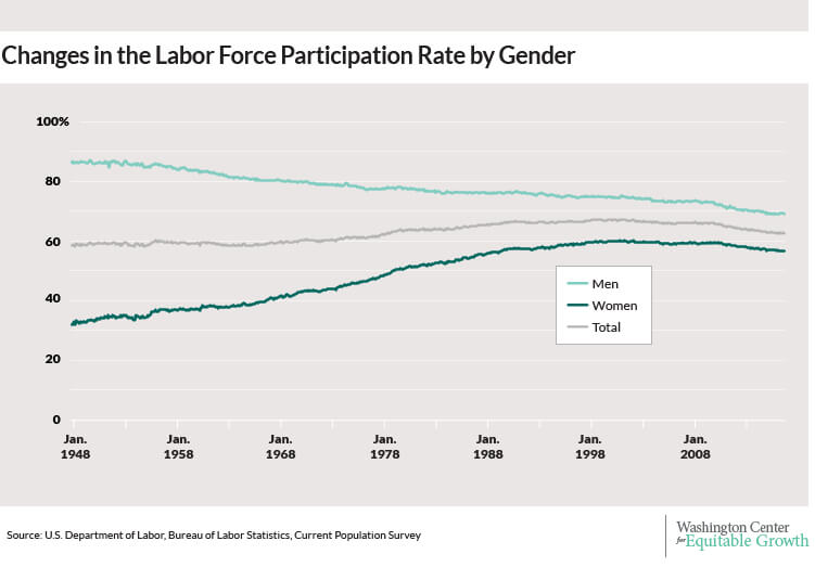
The Bureau of Labor Statistics has been keeping track of the labor force participation rate since January 1948, when the rate was just 58.6 percent. Labor force participation stayed at about this level until 1965 when it began a climb that would last 35 years, until it peaked in April 2000 at 67.3 percent. What caused the steady increase in the rate? Looking at the difference in labor force participation by gender reveals the answer. (See Figure 3.)
Figure 3
The labor force participation rate for men has been on a downward trajectory for nearly 60 years, almost from the moment the agency started keeping track of the statistic. In January 1948, male labor force participation was 86.7 percent. By April 2000, when overall labor force participation peaked, male labor force participation had fallen to 74.9 percent. For women, the trend has operated in precisely the opposite direction. In April 1948, the participation rate for women was 32 percent. Female labor force participation steadily increased for the next half century, peaking at 60.3 percent in April 2000. Over the second half of the 20th century, women moved into the labor force—and were increasingly likely to stay there, even after becoming mothers. This sea change in women’s labor force participation is what helped buoy the overall labor force participation rate, even as men were increasingly less likely to be in the labor force.
Since 2000, however, the growth in women’s labor force participation has stalled out. Men’s labor force participation has continued to decline. So the question remains: what is responsible for the decline beginning in 2000?
The clearest cause of the decline in the overall labor force participation rate is the aging of the population. The Baby Boom generation, born between 1946 and 1964, is a large cohort of workers whose retirement age coincides with decline in labor force participation that began in 2000. As these workers retired, they left the labor force and in turn pushed down the total labor force participation rate.
At the same time, the participation rate for younger workers (age 16 to 24 years) has been on the decline for decades as well. The downward trend in labor force participation for younger Americans is explained by increased schooling: younger workers are more likely to stay in school longer, as college attendance has become substantially more common. So, a positive development—increased educational attainment—pushed down the labor force participation rate.
Yet the demographic shifts described above cannot explain the entire decline in the labor force participation rate. Prime-age workers’ labor force participation has also been on the decline. The rate of participation for workers ages 25 to 54 declined from 84.4 percent in April 2000 to 83.1 percent in December 2007, on the eve of the Great Recession.
Women’s labor force participation was driving the overall upward trend in labor force participation through 2000, so the plateau and then decline in women’s participation in the ensuring years is an important factor for explaining the national trend. Understanding why women’s labor force participation has stalled is key to reversing the downward trends in the national rate. In 1990, the United States had the sixth-highest female labor force participation rate amongst 22 high-income OECD countries. By 2010, its rank had fallen to 17th. Why have other high-income countries continued their climb while the United States has stalled? Research by economists Francine Blau and Lawrence Kahn suggests that the absence of family-friendly policies such as paid parental leave in the United States is responsible for nearly a third of the U.S. decline relative to other OECD economies. As other developed countries have enacted and expanded family-friendly policies, the United States remains the lone developed nation with no paid parental leave.
Trends in labor force participation since the Great Recession
While labor force participation was declining before the Great Recession, the downward trend accelerated during the economic crisis. The raw data cannot tell us how much of the decline since the end of 2007 is a continuation of the longer-term trends discussed above, and how much of the decline is due to the lingering effects of the Great Recession. Untangling these two trends—the structural and the cyclical—has become an important and highly contested debate amongst economists and other labor market analysts.
Some research on the recent decline argues that a large portion was due to the structural forces in place before the recession, and concludes that not much of the current lower rate is due to weakness in the labor market due to the Great Recession. A 2014 study by economist Stephanie Aaronson and her colleagues finds that the majority of the decline is due to structural forces. According to their calculations, cyclical weakness is responsible for pushing down the labor force participation rate between 0.24 and 1 percentage point in the second quarter of 2014. In June 2014, the participation rate was about 3 percentage points below its pre-recession level, meaning the recession was only responsible for, at most, one-third of the lower rate.
Other research finds a much larger role for the recession, albeit over a different time frame. A 2012 study by economist Heidi Shierholz finds that only one-third of the decline between 2007 and 2011 was due to structural factors and the other two-thirds of the decline was due to the cyclical impact of the Great Recession.
An analysis from White House Council of Economic Advisers finds a result somewhere in the middle of these two estimates. The CEA, using conservative estimation techniques, concludes that about half of the decline from 2007 to the middle of 2014 is due to the aging of the population, one-sixth is part of a cyclical decline consistent with what we would expect given previous recessions, and the final third is a combination of other structural trends from before the recession and “consequences of the unique severity of the Great Recession.”
So, while there is room for the rate to move upward as the economy strengthens, long-term forces will continue to exert downward pressure on labor force participation. So far in 2015, the labor force participation rate has been holding fairly steady, moving sideways instead of downward. While the June report saw a 0.3 percentage point decline in the participation rate, we should be cautious about drawing conclusions from this dip. The monthly CPS data are noisy, meaning that several months’ of consistent movement are necessary before concluding that a trend is in place. Drawing conclusions from last month’s numbers is particularly risky, due to an anomaly in the timing of survey data collected by the Bureau of Labor Statistics for the June report.
Policy implications moving forward
What are the implications for future policy? If policy makers want to raise the labor force participation rate, or at least keep it as high as possible, a variety of options belong on the table.
Fiscal and monetary policy that focuses on strengthening economic growth and prioritizing full employment can help boost the labor force participation rate. A new study from economist Jesse Rothstein finds lackluster employment growth across nearly all industries between 2009 and 2014, reflecting a continued shortage of demand for all workers. Stronger economic growth can help pull more workers into the labor force if they see higher wages being offered by employers. Doing so requires more stimulus through fiscal policy, such as increased infrastructure investment. According to the International Monetary Fund, boosting infrastructure spending can accelerate economic growth by 1.5 percent in the short-term. This increased growth would help create jobs and pull discouraged workers back into the labor force, as well as improving the health of the economy in the longer-term. More accommodative monetary policy also has immense potential to stimulate labor demand. Fiscal and monetary policies are immensely important, but smart microeconomic policies could help as well.
First, the absence of family-friendly policies in the United States is a key reason for the decline in the overall labor force participation rate and the stalling out of women’s labor force participation. The Mad Men Era is over, to the great relief of many women. But public policy has not kept up with the needs of working families, and balancing the competing demands of work and home remains a fundamental challenge for millions of households. Recent research suggests that the failure to adapt our policies to meet the demands of the modern American family means that women’s labor force participation has stagnated. Paid family leave, flexible scheduling, affordable high-quality childcare, and universal pre-kindergarten are all policies that could play a major role in jump-starting the engine of women’s labor force participation. By providing policies that recognize individuals’ dual roles as both workers and caregivers, we have the opportunity to attract and retain talent in the labor force.
The potential impact of paid family leave on the labor force participation rate is worth discussing in a bit more detail because of the demographic trends discussed earlier. Research suggests that paid parental leave can substantially improve mothers’ labor force participation, because it encourages them to return to their job following a period of bonding with a new baby. But caregiving extends beyond children, as anyone who has provided care for an aging relative well knows. The share of prime-age workers with eldercare responsibilities is increasing as the Baby Boom cohort ages. Unpaid family caregiving is the most common form of eldercare for people of advanced age. Nearly half of all individuals who provide eldercare are part of the “Sandwich Generation,” simultaneously responsible for both aging parents and young children. Paid family leave that allows workers to take temporary time off to care for a loved one—whether that loved one is a new child or an aging parent—is a potentially powerful tool for bolstering labor force participation.
A second proactive policy option to improve labor force participation is a criminal justice reform agenda that includes a reduction in the incarceration rate and policies to reduce discriminatory employment practices against those with criminal records. The U.S. incarceration rate is currently the highest in the world, a consequence of three decades of dramatic growth in the prison population. While the crime rate has fallen over the same period that the prison population has grown exponentially, research shows that the efficacy of increased incarceration as a crime control technique is virtually non-existent; crime rates rise and fall independent of incarceration rates since the 1990s. Coupled with the rise in incarceration, nearly one in three adults in 2010 had a serious misdemeanor or felony arrest that can show up on a routine background check for employment, and a substantial share of discouraged workers report a felony conviction. Nine in ten large corporations report that they conduct criminal background checks, and a wide range of research suggests that a criminal record (both felony and misdemeanor charges, regardless of age) plays a significant negative role in an individual’s employment prospects. New research by economist Michael Mueller-Smith shows that overly aggressive criminal justice policies can significantly reduce the labor force participation of individuals once they leave prison or jail.
Taken together, the impact of our nation’s current criminal justice policies suggest that reform could play a significant role in improving labor force participation. In the long run, reducing flows into the prison population could help boost the labor force participation rate. In the short-term, “ban the box” policies that remove the criminal history question from job applications and postpone the criminal background check until later in the hiring process could help pull some discouraged workers back into the labor force.
It is important to avoid being distracted by policies that have little to do with the trends in the labor force participation rate. Social Security Disability Insurance, or SSDI, for example, has been cited as a program that reduces the participation rate by discouraging work. Proponents of this hypothesis argue that more relaxed medical screening for disability and an increase in the program’s income-replacement rate have increased the disability rolls and pulled able-bodied workers out of the labor market. But studies suggest that the increase in the number of Americans receiving SSDI may be a simple matter of demographics. For instance, economist Monique Morrisey uses the demographic-adjusted disability incidence rate, which shows that after controlling for the aging of the population the rate for men has been on the decline for the last 20 years. At the same time, the age-adjusted rate for women has increased, but to a level similar to the age-adjusted rate for men. This analysis indicates that disability has not become more prevalent, but rather that the aging of the workforce has been the primary cause of the increase in SSDI receipt. Of course, policymakers may have other reasons for wanting to reform the disability insurance program, but we should not expect changes in SSDI to provide a major boost to the labor force participation rate.
Similarly, the Affordable Care Act has been cited as a program that could reduce the labor force participation rate and depress overall labor supply. To a certain extent, this is true. The Congressional Budget Office’s model predicts that workers will supply less labor once the five-year-old health care law is fully implemented in 2016. Note, however, that this reduction in labor supply is due to choices by the workers, not because of a reduction in employers’ demand for labor. Some of this decline in labor supply will come as a reduction in the hours worked by some workers, rather than a decline in the number of workers employed. In other words, the program may lead to an increase in voluntary part-time work. Data from the past several years shows just that trend: an increase in workers voluntarily working part-time. While the ACA may have impacts on labor supply, those effects generally reflect a positive outcome for workers.
Conclusion
Untangling the causes of causes of labor market trends is a tricky endeavor, particularly given the intersection of a long-run trend with the cataclysmic recession of 2007-2009. The drop in the labor market participation rate means that the unemployment rate overstates the extent of the labor market recovery. While the decline in labor force participation was underway decades before the Great Recession began, the downturn played a significant role in the accelerating the recent decline. Demographic forces, namely the aging of the population, are putting significant downward pressure on the labor force participation rate. While the primacy of demographics means limits the extent to which policies can impact increase labor force participation, this structural challenge does not mean that policy has no role to play. The trick for policymakers is to be strategic, and to pull the levers with the most potential to jump-start the labor market back into high gear.
The last seven years have been disastrous for many workers, particularly for lower-wage workers with little education or formal training, but also for some college-educated and higher-skilled workers. One explanation is that lackluster wage growth and, until recently, high unemployment reflect cyclical conditions—a combination of a lack of demand in the U.S. economy and greater sensitivity of workers on the bottom-rungs of the job ladder to changes in the business cycle. A second explanation attributes stagnant wages and employment losses to structural changes in the labor market, including long-term industrial and demographic shifts and policy changes that reduce the incentive to work. This explanation interprets recent trends as the “new normal” and suggests that the U.S. economy will never return to pre-recession labor market conditions unless policies are changed dramatically.
My research, based on a review of extensive data on labor market outcomes since the end of the Great Recession of 2007-2009, finds no basis for concluding that the recent trend of stagnant wages and low employment is the “new normal.” Rather, the data point to continued business cycle weakness as the most important determinant of workers’ outcomes over the past several years. It is only in the past few months that we have started to see data consistent with growing labor market tightness, and even this trend is too new to be confident. The continued stagnation of wages through the end of 2014 implies that, at a minimum, a fair amount of slack remained in the labor market as of that late date. In turn, policies that would promote faster recoveries and encourage aggregate demand during and after recessions remain key policy tools.
Labor force participation rates are still down sharply since the onset of the Great Recession, but the unemployment rate, which spiked from 5 percent to 9.5 percent during the recession, has almost returned to its pre-recession level. If the low participation rate reflects structural economic changes then the current labor market is the “new normal” and there is not much that policymakers can do to improve short-term performance. If instead the problems are due to cyclical economic weakness, generating continued labor market slack that is hidden by the low unemployment rate, then there is much more scope for fiscal and monetary policy to improve labor market conditions. Clearly, cyclical and structural explanations imply vastly different policy responses.
A number of structural shifts have been suggested as explanations for the “new normal,” among them a reduction in workers’ willingness to take jobs (perhaps driven by changes in the incentives created by government transfer programs such as extended unemployment insurance), an aging population that creates shortages of younger workers, and rapid shifts in employers’ needs toward newer types of skills that are in short supply in the labor force. My examination of recent data finds little basis for any of these hypothesized changes. Rather, the evidence—most notably stagnant wages among those who are employed—suggests that lackluster employment growth from 2009 through at least the end of 2014 reflected a continued shortage of demand for virtually all types of workers. It is only in the most recent data—which may well be a temporary blip—that we start to see wage growth consistent with a tightening labor market. It is far too soon to conclude that structural changes will prevent a full recovery to pre-recession labor force participation rates. In the meantime, it will be important to have accommodative fiscal and monetary policies, lest we strangle the belated, still nascent recovery in its infancy. What little wage growth we have seen to date suggests little reason to worry that increases in demand for labor above the current level will trigger meaningful wage inflation.
What do the data say?
The unemployment rate has been below 6 percent since September 2014, lower than many estimates of the level consistent with “full employment.” (Even in a full-employment labor market, we would expect some unemployment as workers transition from one job to another.) Yet the employment-to-population ratio—the share of working-age adults who hold jobs—has been much slower to recover after the Great Recession, and remains lower than was seen at any point between 1984 and 2009. The difference between these measures of labor market slack reflects a sharp decline since 2007 in the share of the population that is participating in the labor market. These declines have continued throughout the recovery, and show no sign of being reversed.
Diagnoses of the situation have thus depended on which data series one chooses to emphasize. The unemployment rate data suggested a robust recovery from early 2011 onward. By 2014, the economy appeared to have little room left to improve, leading some to conclude that the still low employment rate and weak wage growth must have been the “new normal.” But the employment rate series suggested that there remained substantial slack left in the labor market throughout the period as four percent of the population who had been employed before 2007 but were not being pulled back into the labor market. Neither data series in isolation could reveal the true state of the labor market.
To distinguish between these “glass-half-full” and “glass-half-empty” views, I look to evidence regarding employment and wage growth by industry and demography, seeking indications of imbalances between labor supply and demand. If the labor market in 2013-14 was as tight as the unemployment rate alone indicated then we should have seen wage increases as employers bid against each other for workers who were in increasingly short supply. By contrast, if wage growth remained anemic throughout the period, and if employment shortfalls were spread evenly across high- and low-skill demographic groups, then that would be an indication that the unemployment rate was misleading and that the labor market remained quite slack.
One potential source of structural problems is an imbalance between employers’ needs and the skills being offered by job seekers. Rapid technological changes can lead to increases in the demand for workers with specialized skills, yet slack might still remain in other parts of the labor market. There is clear evidence of this sort of imbalance in the mining and logging sector, which has grown substantially since before the recent recession and where there are clear signs that employers are having trouble finding workers to fill open jobs. But outside of this sector, there is little sign that demand growth has been disproportionately concentrated in sectors such as information and technology that typically require specialized skills.
Rather, job openings have grown most in sectors such as transportation, lodging and food services, and arts and recreation. These data generally appear consistent with the view that the increase in job openings reflects reduced recruiting efforts, lower starting wages, or higher minimum qualifications rather than shortages of qualified workers. (See Figure 1.)
Figure 1
It also is possible that demand for labor within certain industries created shortages of some particular types of workers that are masked by weakness in other subsectors. This explanation is perhaps most plausible for the finance and information sectors, where one can easily imagine shortages of workers with industry-specific skills. The information sector, where technological changes requiring new skills are most likely to be an important component of labor demand, and thus where structural labor supply shortages are most plausible, has had only a modest increase in job openings, and total employment remains below its 2007 level.
Findings by demography
Another source of evidence about mismatches between workers skills’ and firms’ needs lies in the demographic distribution of unemployment. In the recent recession, unemployment rose much more for non-college workers than for those who had attended college, and at each education level more for men than for women. The latter likely reflects the disproportionate declines in construction and manufacturing, which are cyclically sensitive industries that were very hard hit in this cycle. The former could be consistent with a shift in favor of higher-skill workers.
But data from the subsequent economic recovery contradict this explanation. The unemployment rate fell faster in the recovery for less-skilled workers than for college-educated workers, and particularly fast for non-college men. There is no indication that the unemployment rate for college-educated workers has reached any sort of a floor since it remains—even in the most recent data—notably higher than in 2007. (See Figure 2.)
Figure 2
Findings regarding wages
Ultimately, the most decisive way to diagnose the adequacy of labor demand is by examining wages: If employers are having trouble finding suitable workers then they will compete against each other for those workers who are available, bidding up wages. Across-the-board labor shortages would mean increases in wages across the economy while shortages for workers with specialized skills would mean raises in particular sectors.
If the economy were pushing against overall limits then we would expect to see rising wages. But the data through 2014 showed no signs of upward pressure on wages. Average real wages (adjusted for inflation) were stagnant since 2009, with increases below 1 percent per year even in 2014. Workers at the very top of the wage distribution saw larger increases, but even these totaled only 2 to 3 percent between 2008 and 2014, and they were concentrated among the top 20 percent of workers. Below the 80th percentile, real wages fell by about 3 percent at the median. It is only in the most recent data (since the beginning of 2015) where there is any sign of real wage growth, at roughly a 3 percent annual rate. If this is sustained, and especially if it accelerates in the coming months, then it might indicate that the labor market has finally begun to tighten. But a few months of data are too little to support this conclusion, particularly when real wage growth has been boosted by low inflation attributable to declines in energy prices. (See Figure 3.)
Figure 3
Over the longer period, there is no sign of meaningfully larger wage increases in sectors with rising job openings, as would be expected if these sectors faced persistent labor shortages. Across industries, only the mining and finance sectors appear to have posted meaningful wage increases, and even these have averaged less than 1 percent per year real wage growth. Once again, the patterns in the data are fully consistent with continued demand weakness, and not at all consistent with growing shortages of workers in growing sectors. (See Table 1.)
Table 1
Policy implications
In the years since the Great Recession, the unemployment rate has gradually crept downward while other indicators of the health of the labor market have been stagnant. Lackluster wage growth and high unemployment rates among lower-skilled workers appear to be attributable to a continued shortage of demand in the U.S. economy, combined with greater sensitivity to cyclical conditions of workers on the bottom-rungs of the job ladder. That means the high nonemployment rate among lower-skilled workers is not the “new normal” but rather could be substantially resolved by more robust economic growth and better fiscal and monetary demand-management policies.
Further, my research suggests that increased aggregate demand for workers, at the current level, will not create inflation. At best, we are only in the past few months seeing meaningful tightness. More likely, this is an artifact of declining oil prices, which means the current labor market still has substantial slack. Under the latter interpretation, additional labor demand would improve employment outcomes, with particular benefits for low-skilled workers and other disadvantaged groups who suffer disproportionately from cyclical downturns.
My results also counsel against many of the recommendations made by proponents of the view that the economy has settled into a “new normal.” In particular, there are two ill-advised responses to current conditions in the labor market predicated on a misdiagnosis of the economy as having escaped the cyclical downturn. First, tax cuts or reductions in unemployment insurance or means-tested government transfer programs aimed at increasing labor supply will do more to reduce wages than to increase employment.
Second, education and training programs aimed at increasing the skill of low-wage workers are unlikely to do much to help the labor market when there are demand shortages at every rung of the job ladder. So education and training programs are unlikely to help in the short term. That said, these programs alongside increased income support for low earners still make sense as a response to long-term trends—even if they cannot be expected to contribute meaningfully in the short run.
Taking ill-advised policy steps, such as failing to implement needed fiscal and monetary policies to boost demand for labor, or, worse, implementing policies aimed at tamping down an overheating economy, could extend periods of underemployment, damaging workers’ productivity for many years to come. Every month that the economy continues to underperform is making us poorer for decades into the future. Over-cautious policy could cause substantial damage. It is also crucial to put policies in place now to prepare for the next downturn, to avoid such a sustained, weak recovery.
Conclusion
Claims that the economy is nearing its growth potential, and that ongoing low employment rates are the unavoidable consequence of structural changes in the labor market, are at odds with the evidence. Neither comparisons across industries or education groups, nor analyses of wage growth offer any evidence of tight labor markets pushing up against their limits. Unemployment rates remain higher than in 2007 for all ages, education levels, genders, and industries. Sectors that have been more cyclically sensitive in the past saw larger increases in unemployment in the Great Recession, but there is remarkably little difference beyond this observation in the current data. And wages have continued to stagnate for the vast majority of workers, at least until the very most recent data. All of these patterns are consistent with an ongoing shortfall in aggregate labor demand, and less so with a gradual adjustment to technological or demand-driven shocks that created demand for new types of skills that cannot be satisfied by the current workforce.
—Jesse Rothstein is an associate professor of public policy and economics and the director of the Institute for Research on Labor and Employment at the University of California, Berkeley.
The slow-motion economic crisis in Greece finally accelerated into high gear this week, with the imposition of a bank holiday and capital controls following the withholding of another round of capital by the European Central Bank from Greece’s insolvent banks. This is what it looks like when a fixed exchange regime such as the euro fails. To date, the critique of the Eurozone as a system has mostly centered on the inability of an independent central bank to govern an economy as large as Europe’s without also having a European Treasury with tax and spending authority to back it up.
The problems inherent in the Eurozone, however, run deeper than a mismatch between the European Union’s wide monetary and narrow fiscal authority. They can be found in the DNA of the Eurozone. The European Central Bank’s institutional priorities and rules baked in from the start doomed the euro project to eventual failure in exactly this way. The relevant DNA emerged from a strand of the macroeconomic research born in the “neoclassical revolution” of the 1970s. That literature gave intellectual heft to the idea that a central bank should be run completely independent of any democratically-accountable political authority and that the only policy objective a central bank should uphold is to prevent inflation at all costs.
That is how the European Central bank is set up. Its governors are appointed from the central banks of the Eurozone member states and are not subject to any confirmation, as determined by a treaty that supersedes the domestic law of all European Union members. The same treaty requires that the central bank only care about “price stability,” meaning preventing inflation.
The most influential paper undergirding the euro is “Rules Rather Than Discretion: the Inconsistency of Optimal Plans,” published by economists Fynn Kydland of Norway and Edward Prescott of the United States in 1977 (see here for a lucid summary of their work). Their paper is very much a creature of the “stagflation” of the early 1970s. The key idea is that central bankers face a “Time Consistency Problem,” in which no policy they announce will ever be believed.
To understand Kydland and Prescott’s argument, first imagine that unemployment is negatively related to inflation. That is, higher inflation is associated with lower unemployment, and vice versa. Central bankers want to minimize both unemployment and inflation, so they face an inherent tradeoff. Now imagine that the economy exists for only two periods. In the first period, workers and firms form their expectation for inflation in the second period. If the central bank can convince workers and firms in the first period that inflation will be low in the second, then when that second period rolls around the central bank will have a strong incentive to generate surprise inflation in order to lower unemployment. But if workers and firms understand how the game is played, they’ll know a surprise is coming, so they cannot be induced to believe inflation will be low when they form expectations in the first period. Once workers and firms expect high inflation, if the central bank doesn’t deliver it in the second period, then unemployment will be high.
Because of these dynamics around expectations and trust, in the world of Kydland and Prescott’s simple model, an outcome with no inflation and low unemployment is unattainable. Any central banker who tries to reduce unemployment will only end up increasing inflation by inducing workers and firms to expect inflation, which the central banker then has to deliver to avoid unemployment.
To sidestep the Time Consistency Problem, Kydland and Prescott proposed what they called “rules” whereby the central bank should use a mathematical formula to dictate policy, eliminating their discretion. There’s no role for individual central bankers weighing options, hence no opportunity for them to try to fool workers, and hence no concern that workers will be afraid of being fooled and not trust an announced discretionary policy.
As several later writers noted, there’s no guarantee this mathematical formula would not itself be changed, so even mathematically-defined rules based on independent economic data may be just as bad, in practice, as discretion! Instead, as the Time Consistency literature evolved, the critical element in setting anti-inflationary policy is to appoint central bankers with strong reputations for fighting inflation. Everyone will believe them.
The result of this academic wrangling was a consensus in favor of endowing central bankers with no political accountability and tasking them to do whatever’s necessary to curtail inflation should it ever arise. By doing so, they assure inflation never arises in the first place. That is the view that was incorporated into the Maastricht Treaty of 1992 that set up the European Central Bank and gave it the notorious single mandate to reduce inflation, with no eye to mitigating recessions or unemployment.
Inflation has indeed been low in the Eurozone, including in countries such as Spain, Italy, and Greece where inflation had been famously high when these nations had their own currencies and autonomous central banks. But over this same period, inflation has also been low across developed economies, including those without independent central banks (such as the United Kingdom, where the move to independent policymaking only happened in 1997, to no discernible effect), and those with central banks charged with an explicit dual mandate for price stability and full employment (as in the United States).
The problem is that sometimes an economy needs inflation to function well. That’s true of Greece now—a massive debt overhang means that Greek businesses and households aren’t spending. Creditor-enforced austerity means the Greek government isn’t spending either. And an over-valued currency means that no one outside Greece wants to buy what the country is selling.
But the European Central Bank can never allow inflation because in the strange world of the Time Consistency Problem, that would reveal it to be irresponsible and secretly pro-inflation, ultimately leading to hyperinflationary expectations throughout the Eurozone. So despite the massive economic, social, and political cost, the European Central Bank insists on a prolonged depression rather than moderate inflation to work off Greece’s debt overhang. The idea that 25 percent of Greece should be unemployed and the other 75 percent should lose half their income in order to uphold the rigid diktat of an economics paper published in 1977 is not politically sustainable. Instead, Greece may well leave the euro. Either way, the Eurozone will leave its rigid DNA intact. Until the next crisis.
Income inequality in the United States grew more acute in 2014, yet the bottom 99 percent of income earners registered the best real income growth (after factoring in inflation) in 15 years. The latest data from the U.S. Internal Revenue Service show that incomes for the bottom 99 percent of families grew by 3.3 percent over 2013 levels, the best annual growth rate since 1999. But incomes for those families in the top 1 percent of earners grew even faster, by 10.8 percent, over the same period. (See Figure 1.)
Figure 1
Overall, real average incomes per family in 2014 grew by a substantial 4.8 percent. For the bottom 99 percent of income earners, this marks the first year of real recovery from the income losses sparked by the Great Recession of 2007-2009. After a large decline of 11.6 percent from 2007 to 2009, those families saw a negligible 1.1 percent in real income gains from 2009 to 2013. But a full recovery in income growth for the bottom 99 percent is still not in sight. In 2014, these families recovered slightly less than 40 percent of their income losses due to the Great Recession.
Those at or near the top of the income ladder did substantially better in 2014. The share of income going to the top 10 percent of income earners—individuals making an average of $300,000 a year—increased to 49.9 percent in 2014 from 48.9 percent in 2013, the highest ever except for 2012. The share of income going to the top 1 percent of families—those earning on average about $1.3 million a year—increased to 21.2 percent in 2014 from 20.1 percent in 2013. Income inequality, then, remains extremely high, particularly at the very top of the income ladder. (See Figure 2.)
Figure 2
More broadly, the top 1 percent of families captured 58 percent of total real income growth per family from 2009 to 2014, with the bottom 99 percent of families reaping only 42 percent.
The release time for this latest income data from the IRS usually lags behind other key indicators of U.S. economic performance. Aggregate economic growth statistics are typically available a month after the end of each quarter. In contrast, U.S. Census Bureau official income and poverty measures are not available until mid-September of the following year, or 8.5 months after the end of the year. Complete individual income tax statistics, the only statistics that can capture top incomes, are usually not available until 19 months after the end of the year.
This difference in timing explains why economic growth statistics are much more widely discussed than income inequality statistics in public debates about economic inequality and growth. But for the first time, this income data is now more readily available because the Statistics of Income division of the IRS now publishes filing-season statistics by size of income. These statistics can be used to project the distribution of incomes for the full year.
My colleagues and I used these new statistics to update our top income share series for 2014, which are part of our World Top Incomes Database. These statistics measure pre-tax cash market income excluding government transfers such as the disbursal of the earned income tax credit to low-income workers. For the first time, we can produce inequality statistics less than 6 months after the end of the year.
Timely statistics on economic inequality are central to informing the public policy debate about the connections between economic growth and inequality. One case in point: The higher tax rates for top U.S. income earners enacted in 2013 as part of the Obama Administration and Congress’ federal budget deal seem to have had only a fleeting impact on the outsized accumulation of pre-tax income by families in the top 1 percent and 0.1 percent of income earners.
To be sure, there was a shifting of income among high-income earners from 2013 to 2012 as these wealthy families sought to avoid the higher rates enacted in 2013. This adjustment created a spike in the share of top incomes accumulated by the very wealthy in 2012 followed by a trough in 2013. By 2014, however, top incomes shares were back to their upward trajectory. This suggests that the higher tax rates starting in 2013, while not negligible, will not be sufficient by themselves to curb the enormous increase in pre-tax income concentration that has taken place in the United States since the 1970s.
—Emmanuel Saez in a professor of economics at the University of California-Berkeley and a member of the Washington Center for Equitable Growth’s steering committee