If the United States were to invest in a public, voluntary, high-quality universal prekindergarten program starting in 2016 and fully phased in by 2017, what would the long-term impacts be for ? Our study looks to quantify the long-term benefits and costs of investing in a high-quality universal prekindergarten program available to all 3- and 4-year-olds across the United States. Use the data and interactives below to explore how a universal prekindergarten program would affect .
Who would participate?
Currently, in , percent of 3- and 4-year-olds ( children) participate in state-sponsored prekindergarten. Unfortunately, the quality of these programs varies significantly, which means that preschoolers do not always experience the same benefits or long-term effects. If a universal prekindergarten program were enacted in 2016 and fully phased in by 2017, percent of 3- and 4-year-olds ( children) would be enrolled in public prekindergarten, benefiting from a high-quality early childhood education.
What are the benefits of a universal prekindergarten program?
High-quality prekindergarten education can generate significant long-run benefits for participating children, their families, and even other non-participants. Longitudinal studies have shown, for example, that aside from improved educational achievement, children who have attended a prekindergarten program have spent less time in special education and had lower grade retention rates. These children also experience less child maltreatment and reduced crime, smoking, and depression rates over the course of their lives. In addition, both participating children and their parents have higher projected earnings, which subsequently increases government tax revenue.
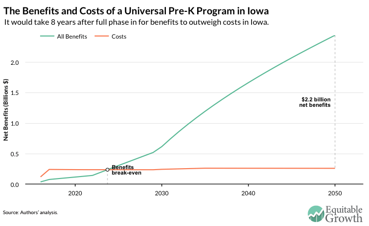
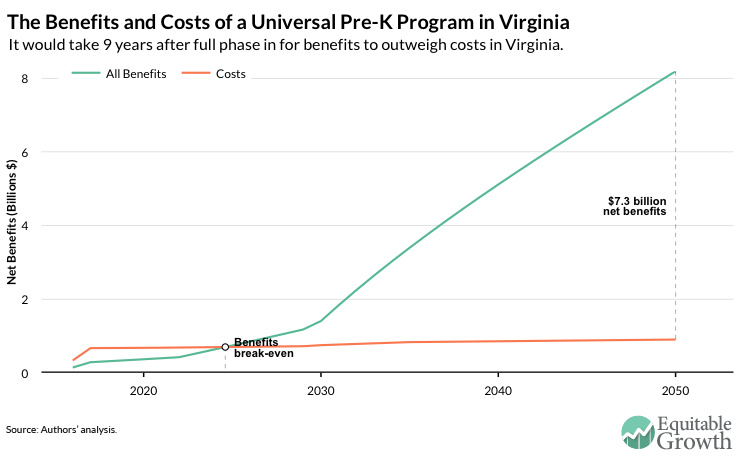
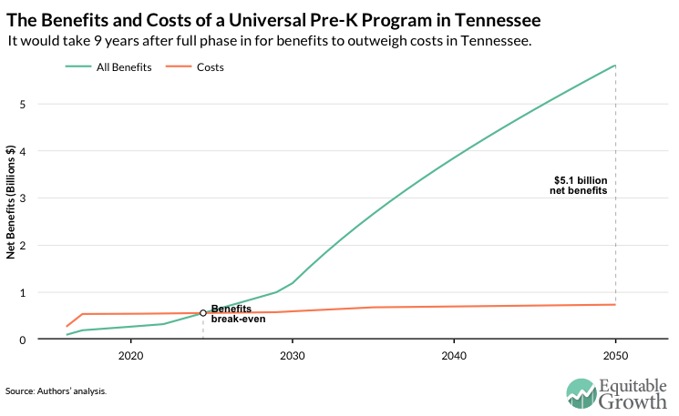
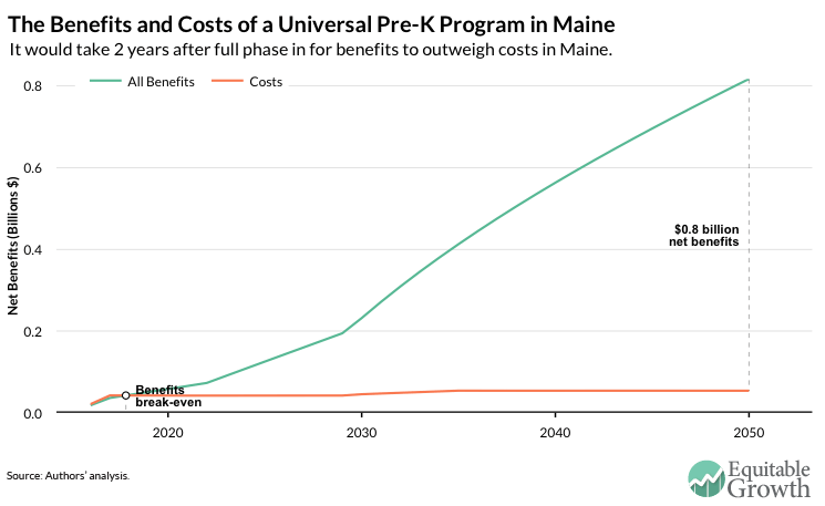
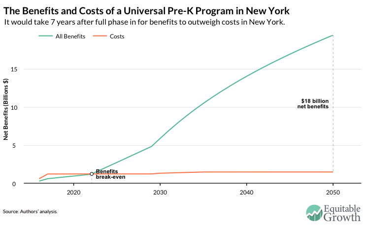
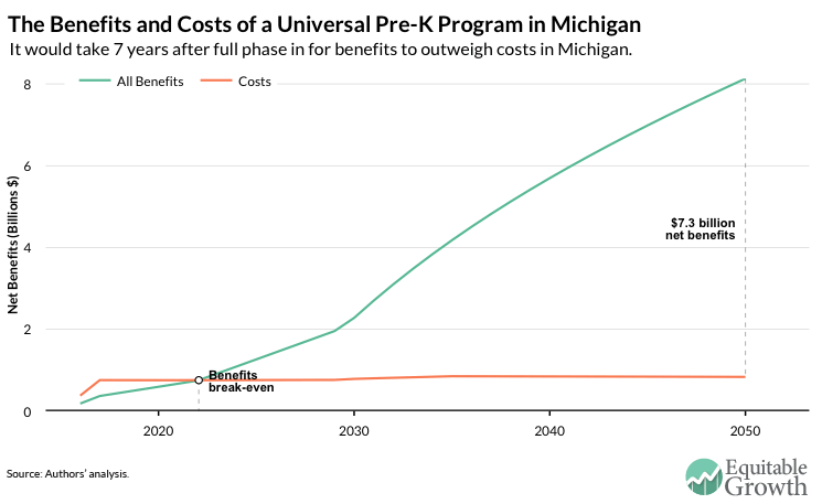
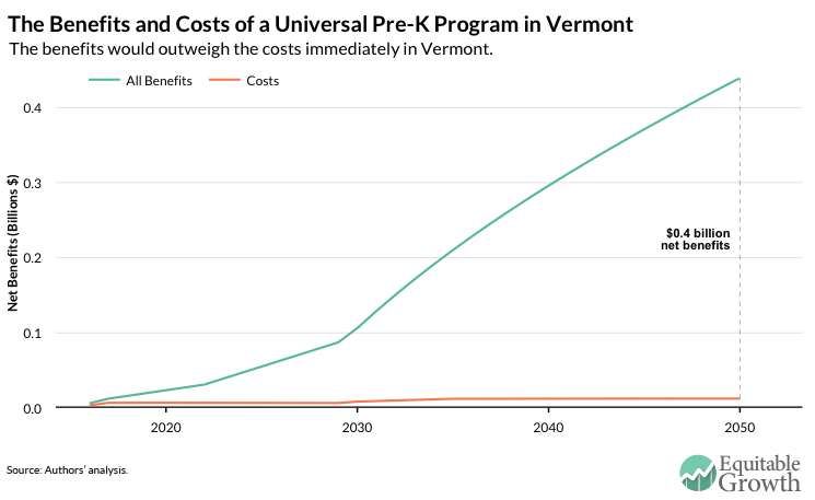
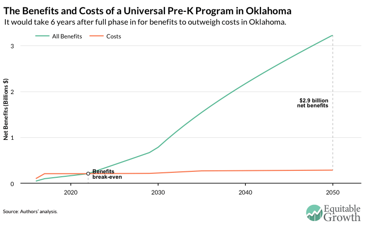
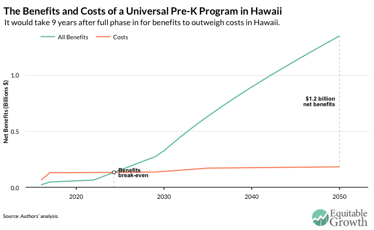
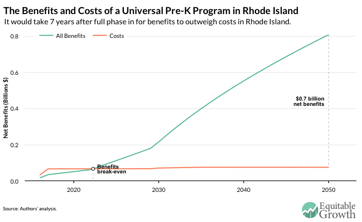
If a universal prekindergarten program were to start in the United States in 2016, would see more than $ million in total benefits in 2050, amounting to savings of $ per capita that year. Here’s how these total benefits break down:
- $ per person is attributed to savings to government.
- $ per person comes from increased compensation.
- The remaining $ per person is accounted for by savings to each individual from better health and less crime.
What are the costs?
Currently, spends $ per capita per year on preschool programs, special education services, and Head Start. In 2017, when a universal prekindergarten program is fully phased in, it would take an investment of $ more per capita per year to maintain a high-quality prekindergarten program.
There are three main costs associated with a high-quality universal prekindergarten program: the cost of the program, increased high school attendance, and increased college attendance. The program itself is based on Chicago’s comprehensive high-quality Child-Parent Center half-day program, so the costs take into account the multitude of services that are provided at the Child-Parent Center offset by the current spending on similar early childhood education programs as to not double-count expenditures. Because studies have shown that students who attend prekindergarten have higher high school completion rates and are more likely to attend college, these usage costs are also factored into the total cost of a universal prekindergarten program.
In 2050, these costs add up to $ million, or $ per capita in . $ per capita is attributed to program costs, $ comes from increased high school usage per person, and the remaining $ per person is accounted for by increased college attendance.
How do the benefits compare to the costs?
If a high-quality universal prekindergarten program were to start in the United States in 2016 and be fully phased in by the end of 2017, the program would require a total of $ million in taxpayer dollars. Over time, the cost would eventually grow to include the cost of additional high school and college attendance. And by 2050, there would be more than $ million in total benefits compared to merely $ million in total costs, yielding net benefits of $ million. By 2050, for every dollar invested in a universal program, there would be $ in returns.
To see the national numbers, return to the full report.