Fact sheet: What do we know about economic inequality and growth?

Overview: Why this matters for policymakers

Recently available research looks across developing and advanced countries and within the United States to examine the effects of economic inequality on economic growth, well-being, and stability.

Research is beginning to find that economic inequality harms economic growth over the long term and that countries with less income and wealth disparities and a larger middle class boast stronger and more stable economic growth. Yes some studies also suggest that in the short run, greater economic inequality may spur growth before hindering it over the longer term. Overall, however, there is growing evidence that more equitable societies are associated with higher rates of long-run growth.

View full fact sheet here alongside all endnotes

Evidence from across states within the United States

Studies that look at the relationship between inequality and growth in the United States mirror those of international studies—less inequality is associated with long-term growth and is particularly associated with lower income growth for those at the top of the income ladder. But the international results also indicate that in the short run economic growth may not be harmed by inequality even in the United States. Here are some key findings:

  •  Ugo Panizza of the U.N. Conference on Trade and Development finds a negative relationship between inequality and growth across U.S. states. A larger share of income accruing to the middle class is associated with higher growth rates, while higher inequality leads to lower growth rates.[i]
  • Using data for 48 states from 1960 to 2000, Mark Partridge of Ohio State University finds that in the short run inequality is positively related to growth while in the long run the income share of the middle class is positively associated with more robust growth.[ii]
  • Economists Mark Frank and Donald Freeman of Sam Houston State University, using methods focusing on longer run trends, find a strong, negative relationship between inequality and growth.[iii] Though, Mark Frank released a subsequent study using new state-level inequality and growth data from 1945 to 2004 that found higher income concentration increased short-run growth. This second paper by Frank highlights some of the nuances of the relationship between inequality and growth.[iv]
  • In a recent book, “Just Growth: Inclusion and Prosperity in America’s Metropolitan Regions,” Chris Benner, associate professor of community and regional development at University of California-Davis, and Manuel Pastor, professor of American studies and ethnicity at University of Southern California, show that less economic inequality within regional economies is linked to regional prosperity.[v]
  • In a 2014 paper by Roy van der Weide of the World Bank and Branko Milanovic of the City University of New York looks at income growth instead of gross domestic product for inequality measures at different points along the income distribution, using state-level data in the United States. They find that high levels of economic inequality decrease income growth for those at the bottom of the income distribution.[vi]
  • Milanovic and van der Weide also find that high levels of inequality at the bottom of the income ladder is associated with slightly faster income growth at the top of the ladder.[vii]
  • Milanovic and van der Weide’s research is consistent with earlier work by then University of Massachusetts-Amherst economist Jeffrey Thompson (now at the Federal Reserve Board in Washington, DC) and Congressional Budget Office analyst Elias Leight, who look at the effects of inequality on incomes across households. They found that increases in the incomes of those at the top of the income ladder, measured by either the top 10 or 1 percent, are associated with declines in incomes of low and middle-income households.[viii]

International comparisons

In the most recent literature of international comparisons, a new, somewhat nuanced theme is emerging that high inequality is bad for economic growth over long time horizons and that high inequality is particularly bad for those on the bottom of the income spectrum. But in the short run, most of the research agrees that high inequality can be associated with faster economic growth, but the benefits tend to flow to the top for that short period of time. Some of the key findings in this research arena include:

  • In May 2015, the Organisation for Economic Co-operation and Development (comprised of developed and leading developing nations) issued its most recent findings in its report “In it together: Why Less Inequality Benefits Us All.” The OECD found that between 1990 and 2010, gross domestic product per person in 19 core OECD countries grew by a total of 28 percent, but would have grown by 33 percent over the same period if inequality had not increased after 1985. The report concludes that “income inequality has a sizeable and statistically significantnegative impact on growth.”[i]
  • To better understand the time dimension of these trends, International Monetary Fund economists Andrew G. Berg and Jonathan D. Ostry looked at periods of growth instead of duration. They find that “countries with more equal income distributions tend to have significantly longer growth spells.” They also found that inequality was a stronger determinant of the quality of economic growth than many other commonly studied factors such as external demand and price shocks, the initial income of the country (did it start out wealthy or very poor?), the institutional makeup of the country, its openness to trade, and its macroeconomic stability.[ii]
  • In a 2014 extension of this work, Ostry, Berg, and their IMF colleague Charalambos Tsangarides include an analysis of the impacts of income redistribution to ameliorate income inequality as well as market inequality. They find that economic growth is lower and periods of growth are shorter in countries that have high inequality as measured by the Gini coefficient of income after taxes and transfer. (The Gini Coefficient is a common measure of income inequality.) In the same paper, the researchers show that transfers (redistributions of income from upper to lower income individuals) do not harm economic growth—at least up to a point consistent with policies in other wealthy nations.[iii]
  • Diego Grijalva of the University of California-Irvine finds that some economic inequality (not extreme inequality though) may have some positive short- and medium-term effects on economic growth, but in the long run high levels of economic inequality tend to be detrimental to economic growth.[iv]
  • Daniel Halter and Josef Zweimuller of the University of Zurich, and Manuel Oechslin of the University of Bern find that there are methodological differences in the papers that find positive relationship between inequality and growth and those that find a negative relationship. Specifically, those papers that examine inequality’s effect on growth over time within countries tend to find a positive relationship but those that use cross-sectional comparisons find a negative relationship. They posit that the time-difference methods are detecting short-term positive effects to growth, while the cross-sectional methods pick up the long-term negative effects for growth when there is persistently high or growing inequality. [v]
  • In 2011, Dan Andrews of the OECD, Christopher Jencks at Harvard University, and Andrew Leigh at Australian National University looked at inequality in the form of concentration of income at the top of the income spectrum (primarily the top 10 percent, but they also tested the top one percent). The results were somewhat contradictory, leading them to conclude that “inequality at the top of the distribution either benefits or harms everyone and therefore depends on long-term effects that we cannot estimate very precisely even with these data.”[vi]

Conclusion

Economic theory supports conflicting narratives about the potential impact of economic inequality on economic growth. There are some ways that inequality could boost growth and other ways that it could retard growth. Furthermore, there are numerous possible mechanisms that could relate inequality to growth and many of these channels would have conflicting outcomes. Because theory cannot provide strong guidance, it is imperative to use data and analysis to understand the relationships.

Studies that look at the longer-term growth implications of economic inequality find that inequality adversely affects growth rates and the duration of periods of growth, while those that focus on short-term growth find that inequality is not harmful and may be associated with faster growth. Furthermore, studies that look at the impact of inequality on different levels of the income distribution find that inequality is particularly bad for the income growth of those not at the top.

Research on inequality and growth may be approaching a new consensus on the general implications of inequality on economic growth, but more work is needed to fully understand the specifics of how inequality affects growth. In particular, now that the United States is approaching a level of inequality that is very rare among developed economies and more closely resembles a developing economy, which mechanisms apply? These are questions that will require continued updates to the data and methods.

View full fact sheet here alongside all endnotes

[i] OECD, In It Together: Why Less Inequality Benefits All (Paris: OECD Publishing, 2015).

[ii] Andrew Berg and Jonathan Ostry, Inequality and Unsustainable Growth (Washington, DC: International Monetary Fund, 2011).

[iii] Jonathan D. Ostry, Andrew Berg, and Charalambos G. Tsangarides, Redistribution, Inequality, and Growth, Discussion Note, IMF Staff Discussion Note (Washington, D.C.: International Monetary Fund, February 2014), http://www.imf.org/external/pubs/ft/sdn/2014/ sdn1402.pdf.

[iv] Diego F. Grijalva, Inequality and Economic Growth: Bridging the Short-Run and the Long-Run, November 29, 2011, http://escholarship.org/uc/item/4kf1t5pb.

[v] Daniel Halter, Manuel Oechslin, and Josef Zweimüller, “Inequality and Growth: The Neglected Time Dimension,” Journal of Economic Growth 19, no. 1 (March 1, 2014): 81–104, doi:10.1007/s10887-013-9099-8.

[vi] Dan Andrews, Christopher Jencks, and Andrew Leigh, “Do Rising Top Incomes Lift All Boats?,” The BE Journal of Economic Analysis & Policy 11, no. 1 (2011), http:// www.degruyter.com/view/j/bejeap.2011.11.issue-1/ bejeap.2011.11.1.2617/bejeap.2011.11.1.2617.xml.

[i] Ugo Panizza, “Income Inequality and Economic Growth: Evidence from American Data,” Journal of Economic Growth 7, no. 1 (2002): 25–41.

[ii] Mark Partridge, “Does Income Distribution Affect U.S. State Economic Growth,” Journal of Regional Science 45 (2005): 363–94.

[iii] Mark W. Frank and Donald Freeman, “Relationship of Inequality to Economic Growth: Evidence from U.S. StateLevel Data,” Pennsylvania Economic Review 11 (2002): 24–36.

[iv] Mark W. Frank, “Inequality and Growth in the United States: Evidence from a New State-Level Panel of Income and Inequality Measures.” Economic Inquiry 47, no. 1 (January 2009): 55–68.

[v] Chris Benner and Manuel Pastor, Just Growth: Inclusion and Prosperity in America’s Metropolitan Regions (New York: Routledge, 2012).

[vi] Van der Weide, Roy, and Branko Milanovic. “Inequality Is Bad for Growth of the Poor (But Not for That of the Rich).” World Bank Policy Research Working Paper 6963 (July 2014). http://www-wds.worldbank.org/servlet/ WDSContentServer/WDSP/IB/2014/07/02/000158349_2 0140702092235/Rendered/PDF/WPS6963.pdf.

[vii] Ibid.

[viii] Jeffrey Thompson and Elias Leight, Searching for the Supposed Benefits of Higher Inequality: Impacts of Rising Top Shares on the Standard of Living of Low and MiddleIncome Families (Amherst: Political Economy Research Institute – University of Massachusetts, Amherst, 2011), http://www.peri.umass.edu/fileadmin/pdf/working_papers/working_papers_251-30.

The Declining Labor Force Participation Rate: Causes, Consequences, and the Path Forward

Elisabeth Jacobs, Senior Director for Policy and Academic Programs, Washington Center for Equitable Growth, testifying before the United States Joint Economic Committee on “What Lower Labor Force Participation Rates Tell Us about Work Opportunities and Incentives”

I would like to thank Chairman Coats, Ranking Member Maloney, and the rest of the Committee for inviting me here today to testify.

My name is Elisabeth Jacobs and I am Senior Director for Policy and Academic Programs at the Washington Center for Equitable Growth. The center is a research and grant-making organization dedicated to understanding what grows our economy, with an emphasis on understanding whether and how economic inequality impacts economic growth and stability.

I am pleased to be here today to address an important topic for understanding the health of the labor market and the economy overall: the labor force participation rate, which currently stands at 62.6 percent. The continued decline of the unemployment rate since 2010 is the most commonly cited piece of evidence that the labor market is recovering. Indeed, it is undeniable that the labor market has improved considerably in the years since the Great Recession, as unemployment has fallen to 5.3 percent, its lowest rate in seven years. Despite this progress, however, the labor market remains troubled. Simply relying on the unemployment rate as an indicator of the health of the job market masks underlying problems, many of which have persisted for decades. In order to fully understand the current state of the labor market, policymakers need to take into account not just the unemployment rate, but also other indicators of how the labor market is functioning, including the labor force participation rate.

My testimony draws five major conclusions:

    • The labor market is recovering from the deepest economic downturn since the Great Depression. The private sector has added 12.8 million private-sector jobs over 64 straight months of job growth, the longest streak of private-sector job creation on record. The unemployment rate is down to 5.3 percent, a seven-year low.
    • While the labor market is on the mend, looking solely at the falling unemployment rate overstates that recovery. Other indicators of labor market health, including the labor force participation rate, suggest that there is more work to be done.
    • The decline in the labor force participation rate predates the Great Recession and is mainly the result of several structural changes in the labor market, including the aging of the workforce.
    • Recent declines in the labor force participation rate that are not explained by long-standing structural changes are largely due to persistent business cycle effects. Five years into the labor market’s recovery from the most severe recession in recent history, demand remains slack.
    • Policy can play an important role in boosting the labor force participation rate, but policymakers need to focus on the correct levers. Persistent slack demand suggests that fiscal and monetary policies are an important first step. In the absence of political action on those fronts, however, family-friendly policies and criminal justice reform are important options.

The rest of my testimony will 1) discuss recent trends in the unemployment rate and other measures of the health of the labor market, 2) examine the potential reasons for the long-run decline in the labor force participation rate, and 3) review the research on the trends in the labor force participation rate since the Great Recession. I conclude by suggesting key implications for policy moving forward.

Download the full pdf for a complete list of sources

Trends in the unemployment rate and the health of the labor market

The Great Recession’s impact on the labor market was devastating. In December 2007, the month the recession began according to the National Bureau of Economic Research, the unemployment rate was 5 percent. By the end of the recession, in June 2009, the unemployment rate hit 9.5 percent and continued to climb until it peaked at 10 percent in October 2009. Over the past five and a half years, the labor market has made substantial progress back toward where it was before the financial crisis. The economy is in the midst of the longest streak of private-sector job growth on record, with 12.8 million jobs created over 64 straight months. The most notable headline has been the continued downward trajectory in the unemployment rate. Joblessness as defined by the official unemployment rate has been on the decline more than 5 years, and stood at 5.3 percent in June, according to the latest data from the Bureau of Labor Statistics. Indeed, an observer looking solely at the unemployment rate might conclude that the labor market is roughly as healthy as it was prior to the Great Recession. (See Figure 1.)

Figure 1

lfpr-testimony-01

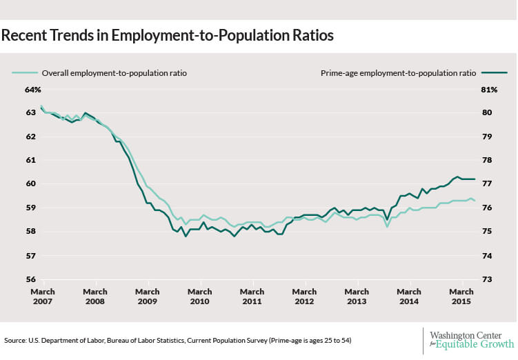
Yet, other measures of the labor market tell a more complicated story. Consider the employment-to-population ratio, which is the share of the total population currently employed. Whereas a decreasing unemployment rate is a sign of improvement in the labor market, an increasing employment ratio can be an even stronger signal of improvement. Unfortunately, the trend in the employment ratio is less sanguine than trend in the unemployment rate.

The employment ratio plummeted during the Great Recession, unsurprisingly. In December 2007, the employment ratio was 62.7 percent, and it fell to a nadir of 58.2 percent in November 2010. The share of the population currently employed has improved over the course of the recovery, and has been growing for just under four years, reaching 59.3 percent in June. Yet it remains 3.4 percentage points below its level prior to the Great Recession, suggesting continued weakness in the labor market. A second key point to keep in mind is that, like many indicators of underlying labor market health, the downward trajectory of the employment ratio pre-dates the Great Recession. The employment ratio peaked in December 2006, a year before the financial crisis, and was higher still in April 2000, when it hit 64.7 percent.

The prime-age employment ratio, or the share of the total population between the ages of 25 and 54 years old with a job, has followed a similar trajectory. Its pre-recession peak, in December 2007, was 79.7 percent. But the prime-age employment ratio was just 77.2 percent in June, a current gap of 2.5 percentage points. The labor market has made considerable gains in the light of the worst recession since the Great Depression. But looking at these employment-to-population ratios is one indication that reveals how those gains are incomplete. (See Figure 2.)

Figure 2

lfpr-testimony-02

Why does the unemployment rate indicate a more complete labor market recovery than does the employment rate? The answer has to do with the intertwined and complicated relationship between the unemployment rate and the labor force participation rate.

The unemployment rate is calculated by the Bureau of Labor Statistics using the Current Population Survey, or CPS, a survey that interviews a sample of households every month and details information about individuals over the age of 16. Individuals who had a job during the week they were interviewed are counted as employed. But not all workers who lack a job are counted as unemployed. According to the CPS, a worker is only officially unemployed if she lacks a job, has actively searched for a job in the last four weeks, and is available to work. Employed workers and officially unemployed workers are together the “labor force.” Any worker without a job who is not counted as officially unemployed is considered to be “not in the labor force.” The official unemployment rate is then calculated by dividing the number of officially unemployed by the labor force. It is an important measure of labor market health because of the clarity of what’s being counted: the unemployment rate is a clear indication of the share of Americans who are actively looking for work. The labor force participation rate is the labor force divided by the total population.

When we think about the unemployment rate declining, we usually think of a situation where an unemployed worker gets a job, moving from unemployment to employment. The ranks of the unemployed would decline, while the size of the labor force would stay the same. The result would be a lower unemployment rate. But the unemployment rate could decline in another way. An unemployed worker could drop out of the labor force, reducing the size of both the number of officially unemployed workers and the labor force. This also would also lead to a decline in the unemployment rate.

An example can help clarify this point. Imagine a labor market with 150 potential workers: 95 are employed, 5 are officially unemployed and 50 are not in the labor force. The official unemployment rate would be 5 percent (5 unemployed workers divided by a labor force of 100 workers.) If one of the unemployed workers got a job, then the unemployment rate would decline to 4 percent (4 unemployed workers divided by a labor force of 100 workers). But if instead an unemployed worker retired and left the labor force, then the unemployment rate would decline to 4.04 percent (4 unemployed workers divided by a labor force of 99 workers). In the first case, the labor force participation rate would stay the same at 66.7 percent (100 divided by 150), but in the second case it would drop to 66 percent (99 divided by 150).

So trends in the unemployment rate are intimately tried to trends in the labor force participation rate. While the decline in the labor force participation rate was particularly stark during the Great Recession, the trend predates it. It’s to the long-term term that I now turn.

The long-run decline in the labor force participation rate

The Bureau of Labor Statistics has been keeping track of the labor force participation rate since January 1948, when the rate was just 58.6 percent. Labor force participation stayed at about this level until 1965 when it began a climb that would last 35 years, until it peaked in April 2000 at 67.3 percent. What caused the steady increase in the rate? Looking at the difference in labor force participation by gender reveals the answer. (See Figure 3.)

Figure 3

lfpr-testimony-03

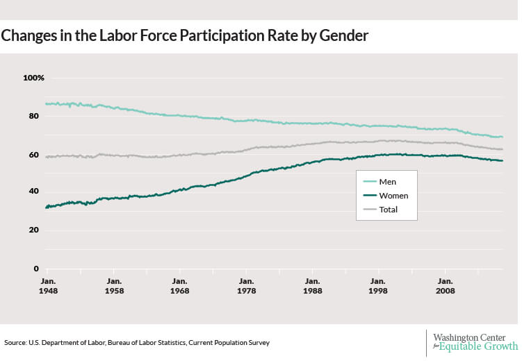
The labor force participation rate for men has been on a downward trajectory for nearly 60 years, almost from the moment the agency started keeping track of the statistic. In January 1948, male labor force participation was 86.7 percent. By April 2000, when overall labor force participation peaked, male labor force participation had fallen to 74.9 percent. For women, the trend has operated in precisely the opposite direction. In April 1948, the participation rate for women was 32 percent. Female labor force participation steadily increased for the next half century, peaking at 60.3 percent in April 2000. Over the second half of the 20th century, women moved into the labor force—and were increasingly likely to stay there, even after becoming mothers. This sea change in women’s labor force participation is what helped buoy the overall labor force participation rate, even as men were increasingly less likely to be in the labor force.

Since 2000, however, the growth in women’s labor force participation has stalled out. Men’s labor force participation has continued to decline. So the question remains: what is responsible for the decline beginning in 2000?

The clearest cause of the decline in the overall labor force participation rate is the aging of the population. The Baby Boom generation, born between 1946 and 1964, is a large cohort of workers whose retirement age coincides with decline in labor force participation that began in 2000. As these workers retired, they left the labor force and in turn pushed down the total labor force participation rate.

At the same time, the participation rate for younger workers  (age 16 to 24 years) has been on the decline for decades as well. The downward trend in labor force participation for younger Americans is explained by increased schooling: younger workers are more likely to stay in school longer, as college attendance has become substantially more common. So, a positive development—increased educational attainment—pushed down the labor force participation rate.

Yet the demographic shifts described above cannot explain the entire decline in the labor force participation rate. Prime-age workers’ labor force participation has also been on the decline. The rate of participation for workers ages 25 to 54 declined from 84.4 percent in April 2000 to 83.1 percent in December 2007, on the eve of the Great Recession.

Women’s labor force participation was driving the overall upward trend in labor force participation through 2000, so the plateau and then decline in women’s participation in the ensuring years is an important factor for explaining the national trend. Understanding why women’s labor force participation has stalled is key to reversing the downward trends in the national rate. In 1990, the United States had the sixth-highest female labor force participation rate amongst 22 high-income OECD countries. By 2010, its rank had fallen to 17th. Why have other high-income countries continued their climb while the United States has stalled? Research by economists Francine Blau and Lawrence Kahn suggests that the absence of family-friendly policies such as paid parental leave in the United States is responsible for nearly a third of the U.S. decline relative to other OECD economies. As other developed countries have enacted and expanded family-friendly policies, the United States remains the lone developed nation with no paid parental leave.

Trends in labor force participation since the Great Recession

While labor force participation was declining before the Great Recession, the downward trend accelerated during the economic crisis. The raw data cannot tell us how much of the decline since the end of 2007 is a continuation of the longer-term trends discussed above, and how much of the decline is due to the lingering effects of the Great Recession. Untangling these two trends—the structural and the cyclical—has become an important and highly contested debate amongst economists and other labor market analysts.

Some research on the recent decline argues that a large portion was due to the structural forces in place before the recession, and concludes that not much of the current lower rate is due to weakness in the labor market due to the Great Recession. A 2014 study by economist Stephanie Aaronson and her colleagues finds that the majority of the decline is due to structural forces. According to their calculations, cyclical weakness is responsible for pushing down the labor force participation rate between 0.24 and 1 percentage point in the second quarter of 2014. In June 2014, the participation rate was about 3 percentage points below its pre-recession level, meaning the recession was only responsible for, at most, one-third of the lower rate.

Other research finds a much larger role for the recession, albeit over a different time frame. A 2012 study by economist Heidi Shierholz finds that only one-third of the decline between 2007 and 2011 was due to structural factors and the other two-thirds of the decline was due to the cyclical impact of the Great Recession.

An analysis from White House Council of Economic Advisers finds a result somewhere in the middle of these two estimates. The CEA, using conservative estimation techniques, concludes that about half of the decline from 2007 to the middle of 2014 is due to the aging of the population, one-sixth is part of a cyclical decline consistent with what we would expect given previous recessions, and the final third is a combination of other structural trends from before the recession and “consequences of the unique severity of the Great Recession.”

So, while there is room for the rate to move upward as the economy strengthens, long-term forces will continue to exert downward pressure on labor force participation. So far in 2015, the labor force participation rate has been holding fairly steady, moving sideways instead of downward. While the June report saw a 0.3 percentage point decline in the participation rate, we should be cautious about drawing conclusions from this dip. The monthly CPS data are noisy, meaning that several months’ of consistent movement are necessary before concluding that a trend is in place. Drawing conclusions from last month’s numbers is particularly risky, due to an anomaly in the timing of survey data collected by the Bureau of Labor Statistics for the June report.

Policy implications moving forward

What are the implications for future policy? If policy makers want to raise the labor force participation rate, or at least keep it as high as possible, a variety of options belong on the table.

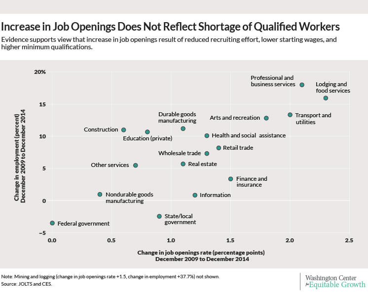
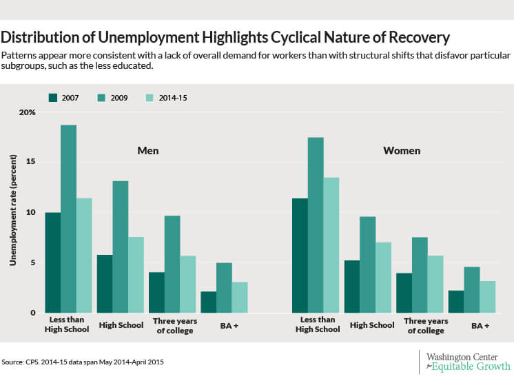
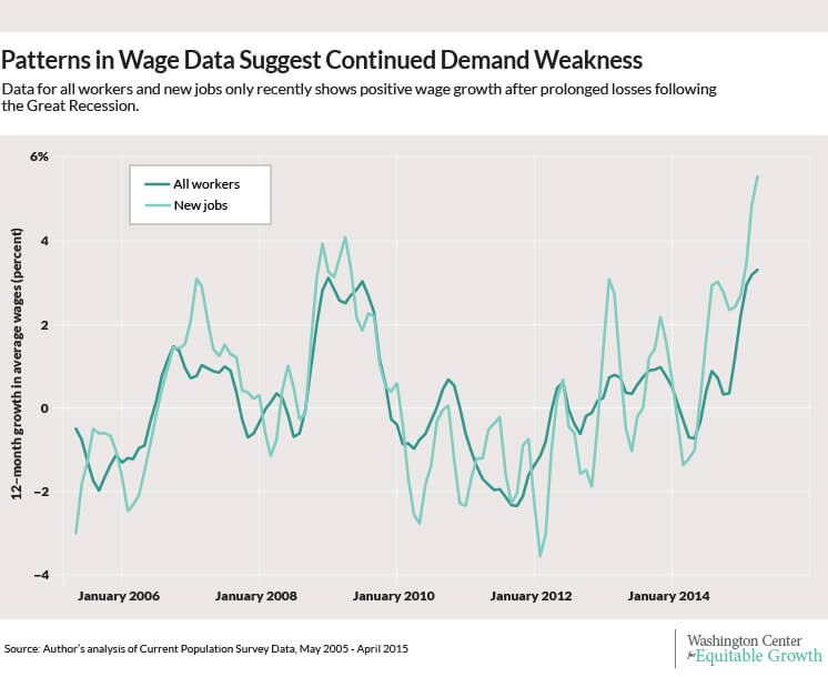
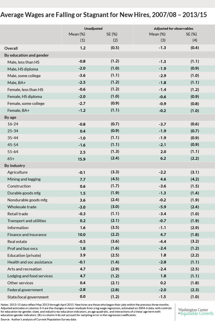
Fiscal and monetary policy that focuses on strengthening economic growth and prioritizing full employment can help boost the labor force participation rate. A new study from economist Jesse Rothstein finds lackluster employment growth across nearly all industries between 2009 and 2014, reflecting a continued shortage of demand for all workers. Stronger economic growth can help pull more workers into the labor force if they see higher wages being offered by employers. Doing so requires more stimulus through fiscal policy, such as increased infrastructure investment. According to the International Monetary Fund, boosting infrastructure spending can accelerate economic growth by 1.5 percent in the short-term. This increased growth would help create jobs and pull discouraged workers back into the labor force, as well as improving the health of the economy in the longer-term. More accommodative monetary policy also has immense potential to stimulate labor demand. Fiscal and monetary policies are immensely important, but smart microeconomic policies could help as well.

First, the absence of family-friendly policies in the United States is a key reason for the decline in the overall labor force participation rate and the stalling out of women’s labor force participation. The Mad Men Era is over, to the great relief of many women. But public policy has not kept up with the needs of working families, and balancing the competing demands of work and home remains a fundamental challenge for millions of households. Recent research suggests that the failure to adapt our policies to meet the demands of the modern American family means that women’s labor force participation has stagnated. Paid family leave, flexible scheduling, affordable high-quality childcare, and universal pre-kindergarten are all policies that could play a major role in jump-starting the engine of women’s labor force participation. By providing policies that recognize individuals’ dual roles as both workers and caregivers, we have the opportunity to attract and retain talent in the labor force.

The potential impact of paid family leave on the labor force participation rate is worth discussing in a bit more detail because of the demographic trends discussed earlier. Research suggests that paid parental leave can substantially improve mothers’ labor force participation, because it encourages them to return to their job following a period of bonding with a new baby. But caregiving extends beyond children, as anyone who has provided care for an aging relative well knows. The share of prime-age workers with eldercare responsibilities is increasing as the Baby Boom cohort ages. Unpaid family caregiving is the most common form of eldercare for people of advanced age. Nearly half of all individuals who provide eldercare are part of the “Sandwich Generation,” simultaneously responsible for both aging parents and young children. Paid family leave that allows workers to take temporary time off to care for a loved one—whether that loved one is a new child or an aging parent—is a potentially powerful tool for bolstering labor force participation.

A second proactive policy option to improve labor force participation is a criminal justice reform agenda that includes a reduction in the incarceration rate and policies to reduce discriminatory employment practices against those with criminal records. The U.S. incarceration rate is currently the highest in the world, a consequence of three decades of dramatic growth in the prison population. While the crime rate has fallen over the same period that the prison population has grown exponentially, research shows that the efficacy of increased incarceration as a crime control technique is virtually non-existent; crime rates rise and fall independent of incarceration rates since the 1990s. Coupled with the rise in incarceration, nearly one in three adults in 2010 had a serious misdemeanor or felony arrest that can show up on a routine background check for employment, and a substantial share of discouraged workers report a felony conviction. Nine in ten large corporations report that they conduct criminal background checks, and a wide range of research suggests that a criminal record (both felony and misdemeanor charges, regardless of age) plays a significant negative role in an individual’s employment prospects. New research by economist Michael Mueller-Smith shows that overly aggressive criminal justice policies can significantly reduce the labor force participation of individuals once they leave prison or jail.

Taken together, the impact of our nation’s current criminal justice policies suggest that reform could play a significant role in improving labor force participation. In the long run, reducing flows into the prison population could help boost the labor force participation rate. In the short-term, “ban the box” policies that remove the criminal history question from job applications and postpone the criminal background check until later in the hiring process could help pull some discouraged workers back into the labor force.

It is important to avoid being distracted by policies that have little to do with the trends in the labor force participation rate. Social Security Disability Insurance, or SSDI, for example, has been cited as a program that reduces the participation rate by discouraging work. Proponents of this hypothesis argue that more relaxed medical screening for disability and an increase in the program’s income-replacement rate have increased the disability rolls and pulled able-bodied workers out of the labor market. But studies suggest that the increase in the number of Americans receiving SSDI may be a simple matter of demographics. For instance, economist Monique Morrisey uses the demographic-adjusted disability incidence rate, which shows that after controlling for the aging of the population the rate for men has been on the decline for the last 20 years. At the same time, the age-adjusted rate for women has increased, but to a level similar to the age-adjusted rate for men. This analysis indicates that disability has not become more prevalent, but rather that the aging of the workforce has been the primary cause of the increase in SSDI receipt. Of course, policymakers may have other reasons for wanting to reform the disability insurance program, but we should not expect changes in SSDI to provide a major boost to the labor force participation rate.

Similarly, the Affordable Care Act has been cited as a program that could reduce the labor force participation rate and depress overall labor supply. To a certain extent, this is true. The Congressional Budget Office’s model predicts that workers will supply less labor once the five-year-old health care law is fully implemented in 2016. Note, however, that this reduction in labor supply is due to choices by the workers, not because of a reduction in employers’ demand for labor. Some of this decline in labor supply will come as a reduction in the hours worked by some workers, rather than a decline in the number of workers employed. In other words, the program may lead to an increase in voluntary part-time work. Data from the past several years shows just that trend: an increase in workers voluntarily working part-time. While the ACA may have impacts on labor supply, those effects generally reflect a positive outcome for workers.

Conclusion

Untangling the causes of causes of labor market trends is a tricky endeavor, particularly given the intersection of a long-run trend with the cataclysmic recession of 2007-2009. The drop in the labor market participation rate means that the unemployment rate overstates the extent of the labor market recovery. While the decline in labor force participation was underway decades before the Great Recession began, the downturn played a significant role in the accelerating the recent decline. Demographic forces, namely the aging of the population, are putting significant downward pressure on the labor force participation rate. While the primacy of demographics means limits the extent to which policies can impact increase labor force participation, this structural challenge does not mean that policy has no role to play. The trick for policymakers is to be strategic, and to pull the levers with the most potential to jump-start the labor market back into high gear.

The Great Recession and its aftermath: What role do structural changes play?

The last seven years have been disastrous for many workers, particularly for lower-wage workers with little education or formal training, but also for some college-educated and higher-skilled workers. One explanation is that lackluster wage growth and, until recently, high unemployment reflect cyclical conditions—a combination of a lack of demand in the U.S. economy and greater sensitivity of workers on the bottom-rungs of the job ladder to changes in the business cycle. A second explanation attributes stagnant wages and employment losses to structural changes in the labor market, including long-term industrial and demographic shifts and policy changes that reduce the incentive to work. This explanation interprets recent trends as the “new normal” and suggests that the U.S. economy will never return to pre-recession labor market conditions unless policies are changed dramatically.

My research, based on a review of extensive data on labor market outcomes since the end of the Great Recession of 2007-2009, finds no basis for concluding that the recent trend of stagnant wages and low employment is the “new normal.” Rather, the data point to continued business cycle weakness as the most important determinant of workers’ outcomes over the past several years. It is only in the past few months that we have started to see data consistent with growing labor market tightness, and even this trend is too new to be confident. The continued stagnation of wages through the end of 2014 implies that, at a minimum, a fair amount of slack remained in the labor market as of that late date. In turn, policies that would promote faster recoveries and encourage aggregate demand during and after recessions remain key policy tools.

View full pdf here.

Why is this relevant for policymakers?

Labor force participation rates are still down sharply since the onset of the Great Recession, but the unemployment rate, which spiked from 5 percent to 9.5 percent during the recession, has almost returned to its pre-recession level. If the low participation rate reflects structural economic changes then the current labor market is the “new normal” and there is not much that policymakers can do to improve short-term performance. If instead the problems are due to cyclical economic weakness, generating continued labor market slack that is hidden by the low unemployment rate, then there is much more scope for fiscal and monetary policy to improve labor market conditions. Clearly, cyclical and structural explanations imply vastly different policy responses.

A number of structural shifts have been suggested as explanations for the “new normal,” among them a reduction in workers’ willingness to take jobs (perhaps driven by changes in the incentives created by government transfer programs such as extended unemployment insurance), an aging population that creates shortages of younger workers, and rapid shifts in employers’ needs toward newer types of skills that are in short supply in the labor force. My examination of recent data finds little basis for any of these hypothesized changes. Rather, the evidence—most notably stagnant wages among those who are employed—suggests that lackluster employment growth from 2009 through at least the end of 2014 reflected a continued shortage of demand for virtually all types of workers. It is only in the most recent data—which may well be a temporary blip—that we start to see wage growth consistent with a tightening labor market. It is far too soon to conclude that structural changes will prevent a full recovery to pre-recession labor force participation rates. In the meantime, it will be important to have accommodative fiscal and monetary policies, lest we strangle the belated, still nascent recovery in its infancy. What little wage growth we have seen to date suggests little reason to worry that increases in demand for labor above the current level will trigger meaningful wage inflation.

What do the data say?

The unemployment rate has been below 6 percent since September 2014, lower than many estimates of the level consistent with “full employment.” (Even in a full-employment labor market, we would expect some unemployment as workers transition from one job to another.) Yet the employment-to-population ratio—the share of working-age adults who hold jobs—has been much slower to recover after the Great Recession, and remains lower than was seen at any point between 1984 and 2009. The difference between these measures of labor market slack reflects a sharp decline since 2007 in the share of the population that is participating in the labor market. These declines have continued throughout the recovery, and show no sign of being reversed.

Diagnoses of the situation have thus depended on which data series one chooses to emphasize. The unemployment rate data suggested a robust recovery from early 2011 onward. By 2014, the economy appeared to have little room left to improve, leading some to conclude that the still low employment rate and weak wage growth must have been the “new normal.” But the employment rate series suggested that there remained substantial slack left in the labor market throughout the period as four percent of the population who had been employed before 2007 but were not being pulled back into the labor market. Neither data series in isolation could reveal the true state of the labor market.

To distinguish between these “glass-half-full” and “glass-half-empty” views, I look to evidence regarding employment and wage growth by industry and demography, seeking indications of imbalances between labor supply and demand. If the labor market in 2013-14 was as tight as the unemployment rate alone indicated then we should have seen wage increases as employers bid against each other for workers who were in increasingly short supply. By contrast, if wage growth remained anemic throughout the period, and if employment shortfalls were spread evenly across high- and low-skill demographic groups, then that would be an indication that the unemployment rate was misleading and that the labor market remained quite slack.

View full pdf here.

Findings by industry

One potential source of structural problems is an imbalance between employers’ needs and the skills being offered by job seekers. Rapid technological changes can lead to increases in the demand for workers with specialized skills, yet slack might still remain in other parts of the labor market. There is clear evidence of this sort of imbalance in the mining and logging sector, which has grown substantially since before the recent recession and where there are clear signs that employers are having trouble finding workers to fill open jobs. But outside of this sector, there is little sign that demand growth has been disproportionately concentrated in sectors such as information and technology that typically require specialized skills.

Rather, job openings have grown most in sectors such as transportation, lodging and food services, and arts and recreation. These data generally appear consistent with the view that the increase in job openings reflects reduced recruiting efforts, lower starting wages, or higher minimum qualifications rather than shortages of qualified workers.  (See Figure 1.)

Figure 1

070615-rothstein-ib-web-02

It also is possible that demand for labor within certain industries created shortages of some particular types of workers that are masked by weakness in other subsectors. This explanation is perhaps most plausible for the finance and information sectors, where one can easily imagine shortages of workers with industry-specific skills. The information sector, where technological changes requiring new skills are most likely to be an important component of labor demand, and thus where structural labor supply shortages are most plausible, has had only a modest increase in job openings, and total employment remains below its 2007 level.

Findings by demography

Another source of evidence about mismatches between workers skills’ and firms’ needs lies in the demographic distribution of unemployment. In the recent recession, unemployment rose much more for non-college workers than for those who had attended college, and at each education level more for men than for women. The latter likely reflects the disproportionate declines in construction and manufacturing, which are cyclically sensitive industries that were very hard hit in this cycle. The former could be consistent with a shift in favor of higher-skill workers.

But data from the subsequent economic recovery contradict this explanation. The unemployment rate fell faster in the recovery for less-skilled workers than for college-educated workers, and particularly fast for non-college men. There is no indication that the unemployment rate for college-educated workers has reached any sort of a floor since it remains—even in the most recent data—notably higher than in 2007. (See Figure 2.)

Figure 2

070615-rothstein-ib-web-01

Findings regarding wages

Ultimately, the most decisive way to diagnose the adequacy of labor demand is by examining wages: If employers are having trouble finding suitable workers then they will compete against each other for those workers who are available, bidding up wages. Across-the-board labor shortages would mean increases in wages across the economy while shortages for workers with specialized skills would mean raises in particular sectors.

If the economy were pushing against overall limits then we would expect to see rising wages. But the data through 2014 showed no signs of upward pressure on wages. Average real wages (adjusted for inflation) were stagnant since 2009, with increases below 1 percent per year even in 2014. Workers at the very top of the wage distribution saw larger increases, but even these totaled only 2 to 3 percent between 2008 and 2014, and they were concentrated among the top 20 percent of workers. Below the 80th percentile, real wages fell by about 3 percent at the median. It is only in the most recent data (since the beginning of 2015) where there is any sign of real wage growth, at roughly a 3 percent annual rate. If this is sustained, and especially if it accelerates in the coming months, then it might indicate that the labor market has finally begun to tighten. But a few months of data are too little to support this conclusion, particularly when real wage growth has been boosted by low inflation attributable to declines in energy prices. (See Figure 3.)

Figure 3

070615-rothstein-ib-web-03

Over the longer period, there is no sign of meaningfully larger wage increases in sectors with rising job openings, as would be expected if these sectors faced persistent labor shortages. Across industries, only the mining and finance sectors appear to have posted meaningful wage increases, and even these have averaged less than 1 percent per year real wage growth. Once again, the patterns in the data are fully consistent with continued demand weakness, and not at all consistent with growing shortages of workers in growing sectors. (See Table 1.)

Table 1

070615-rothstein-ib-web-04

Policy implications

In the years since the Great Recession, the unemployment rate has gradually crept downward while other indicators of the health of the labor market have been stagnant. Lackluster wage growth and high unemployment rates among lower-skilled workers appear to be attributable to a continued shortage of demand in the U.S. economy, combined with greater sensitivity to cyclical conditions of workers on the bottom-rungs of the job ladder. That means the high nonemployment rate among lower-skilled workers is not the “new normal” but rather could be substantially resolved by more robust economic growth and better fiscal and monetary demand-management policies.

Further, my research suggests that increased aggregate demand for workers, at the current level, will not create inflation. At best, we are only in the past few months seeing meaningful tightness. More likely, this is an artifact of declining oil prices, which means the current labor market still has substantial slack. Under the latter interpretation, additional labor demand would improve employment outcomes, with particular benefits for low-skilled workers and other disadvantaged groups who suffer disproportionately from cyclical downturns.

My results also counsel against many of the recommendations made by proponents of the view that the economy has settled into a “new normal.” In particular, there are two ill-advised responses to current conditions in the labor market predicated on a misdiagnosis of the economy as having escaped the cyclical downturn. First, tax cuts or reductions in unemployment insurance or means-tested government transfer programs aimed at increasing labor supply will do more to reduce wages than to increase employment.

Second, education and training programs aimed at increasing the skill of low-wage workers are unlikely to do much to help the labor market when there are demand shortages at every rung of the job ladder. So education and training programs are unlikely to help in the short term. That said, these programs alongside increased income support for low earners still make sense as a response to long-term trends—even if they cannot be expected to contribute meaningfully in the short run.

Taking ill-advised policy steps, such as failing to implement needed fiscal and monetary policies to boost demand for labor, or, worse, implementing policies aimed at tamping down an overheating economy, could extend periods of underemployment, damaging workers’ productivity for many years to come. Every month that the economy continues to underperform is making us poorer for decades into the future. Over-cautious policy could cause substantial damage. It is also crucial to put policies in place now to prepare for the next downturn, to avoid such a sustained, weak recovery.

Conclusion

Claims that the economy is nearing its growth potential, and that ongoing low employment rates are the unavoidable consequence of structural changes in the labor market, are at odds with the evidence. Neither comparisons across industries or education groups, nor analyses of wage growth offer any evidence of tight labor markets pushing up against their limits. Unemployment rates remain higher than in 2007 for all ages, education levels, genders, and industries. Sectors that have been more cyclically sensitive in the past saw larger increases in unemployment in the Great Recession, but there is remarkably little difference beyond this observation in the current data. And wages have continued to stagnate for the vast majority of workers, at least until the very most recent data. All of these patterns are consistent with an ongoing shortfall in aggregate labor demand, and less so with a gradual adjustment to technological or demand-driven shocks that created demand for new types of skills that cannot be satisfied by the current workforce.

—Jesse Rothstein is an associate professor of public policy and economics and the director of the Institute for Research on Labor and Employment at the University of California, Berkeley.

View full pdf here.

The rigid DNA of the European Central Bank

The slow-motion economic crisis in Greece finally accelerated into high gear this week, with the imposition of a bank holiday and capital controls following the withholding of another round of capital by the European Central Bank from Greece’s insolvent banks. This is what it looks like when a fixed exchange regime such as the euro fails. To date, the critique of the Eurozone as a system has mostly centered on the inability of an independent central bank to govern an economy as large as Europe’s without also having a European Treasury with tax and spending authority to back it up.

The problems inherent in the Eurozone, however, run deeper than a mismatch between the European Union’s wide monetary and narrow fiscal authority. They can be found in the DNA of the Eurozone. The European Central Bank’s institutional priorities and rules baked in from the start doomed the euro project to eventual failure in exactly this way. The relevant DNA emerged from a strand of the macroeconomic research born in the “neoclassical revolution” of the 1970s. That literature gave intellectual heft to the idea that a central bank should be run completely independent of any democratically-accountable political authority and that the only policy objective a central bank should uphold is to prevent inflation at all costs.

That is how the European Central bank is set up. Its governors are appointed from the central banks of the Eurozone member states and are not subject to any confirmation, as determined by a treaty that supersedes the domestic law of all European Union members. The same treaty requires that the central bank only care about “price stability,” meaning preventing inflation.

The most influential paper undergirding the euro is “Rules Rather Than Discretion: the Inconsistency of Optimal Plans,” published by economists Fynn Kydland of Norway and Edward Prescott of the United States in 1977 (see here for a lucid summary of their work). Their paper is very much a creature of the “stagflation” of the early 1970s. The key idea is that central bankers face a “Time Consistency Problem,” in which no policy they announce will ever be believed.

To understand Kydland and Prescott’s argument, first imagine that unemployment is negatively related to inflation. That is, higher inflation is associated with lower unemployment, and vice versa. Central bankers want to minimize both unemployment and inflation, so they face an inherent tradeoff. Now imagine that the economy exists for only two periods. In the first period, workers and firms form their expectation for inflation in the second period. If the central bank can convince workers and firms in the first period that inflation will be low in the second, then when that second period rolls around the central bank will have a strong incentive to generate surprise inflation in order to lower unemployment. But if workers and firms understand how the game is played, they’ll know a surprise is coming, so they cannot be induced to believe inflation will be low when they form expectations in the first period. Once workers and firms expect high inflation, if the central bank doesn’t deliver it in the second period, then unemployment will be high.

Because of these dynamics around expectations and trust, in the world of Kydland and Prescott’s simple model, an outcome with no inflation and low unemployment is unattainable. Any central banker who tries to reduce unemployment will only end up increasing inflation by inducing workers and firms to expect inflation, which the central banker then has to deliver to avoid unemployment.

To sidestep the Time Consistency Problem, Kydland and Prescott proposed what they called “rules” whereby the central bank should use a mathematical formula to dictate policy, eliminating their discretion. There’s no role for individual central bankers weighing options, hence no opportunity for them to try to fool workers, and hence no concern that workers will be afraid of being fooled and not trust an announced discretionary policy.

As several later writers noted, there’s no guarantee this mathematical formula would not itself be changed, so even mathematically-defined rules based on independent economic data may be just as bad, in practice, as discretion! Instead, as the Time Consistency literature evolved, the critical element in setting anti-inflationary policy is to appoint central bankers with strong reputations for fighting inflation. Everyone will believe them.

The result of this academic wrangling was a consensus in favor of endowing central bankers with no political accountability and tasking them to do whatever’s necessary to curtail inflation should it ever arise. By doing so, they assure inflation never arises in the first place. That is the view that was incorporated into the Maastricht Treaty of 1992 that set up the European Central Bank and gave it the notorious single mandate to reduce inflation, with no eye to mitigating recessions or unemployment.

Inflation has indeed been low in the Eurozone, including in countries such as Spain, Italy, and Greece where inflation had been famously high when these nations had their own currencies and autonomous central banks. But over this same period, inflation has also been low across developed economies, including those without independent central banks (such as the United Kingdom, where the move to independent policymaking only happened in 1997, to no discernible effect), and those with central banks charged with an explicit dual mandate for price stability and full employment (as in the United States).

The problem is that sometimes an economy needs inflation to function well. That’s true of Greece now—a massive debt overhang means that Greek businesses and households aren’t spending. Creditor-enforced austerity means the Greek government isn’t spending either. And an over-valued currency means that no one outside Greece wants to buy what the country is selling.

But the European Central Bank can never allow inflation because in the strange world of the Time Consistency Problem, that would reveal it to be irresponsible and secretly pro-inflation, ultimately leading to hyperinflationary expectations throughout the Eurozone. So despite the massive economic, social, and political cost, the European Central Bank insists on a prolonged depression rather than moderate inflation to work off Greece’s debt overhang. The idea that 25 percent of Greece should be unemployed and the other 75 percent should lose half their income in order to uphold the rigid diktat of an economics paper published in 1977 is not politically sustainable. Instead, Greece may well leave the euro. Either way, the Eurozone will leave its rigid DNA intact. Until the next crisis.

U.S. income inequality persists amid overall growth in 2014

Income inequality in the United States grew more acute in 2014, yet the bottom 99 percent of income earners registered the best real income growth (after factoring in inflation) in 15 years. The latest data from the U.S. Internal Revenue Service show that incomes for the bottom 99 percent of families grew by 3.3 percent over 2013 levels, the best annual growth rate since 1999. But incomes for those families in the top 1 percent of earners grew even faster, by 10.8 percent, over the same period. (See Figure 1.)

Figure 1

Saez1_6262015

Overall, real average incomes per family in 2014 grew by a substantial 4.8 percent. For the bottom 99 percent of income earners, this marks the first year of real recovery from the income losses sparked by the Great Recession of 2007-2009. After a large decline of 11.6 percent from 2007 to 2009, those families saw a negligible 1.1 percent in real income gains from 2009 to 2013. But a full recovery in income growth for the bottom 99 percent is still not in sight. In 2014, these families recovered slightly less than 40 percent of their income losses due to the Great Recession.

Those at or near the top of the income ladder did substantially better in 2014. The share of income going to the top 10 percent of income earners—individuals making an average of $300,000 a year—increased to 49.9 percent in 2014 from 48.9 percent in 2013, the highest ever except for 2012. The share of income going to the top 1 percent of families—those earning on average about $1.3 million a year—increased to 21.2 percent in 2014 from 20.1 percent in 2013. Income inequality, then, remains extremely high, particularly at the very top of the income ladder. (See Figure 2.)

Figure 2

Saez2_6262015

More broadly, the top 1 percent of families captured 58 percent of total real income growth per family from 2009 to 2014, with the bottom 99 percent of families reaping only 42 percent.

The release time for this latest income data from the IRS usually lags behind other key indicators of U.S. economic performance. Aggregate economic growth statistics are typically available a month after the end of each quarter. In contrast, U.S. Census Bureau official income and poverty measures are not available until mid-September of the following year, or 8.5 months after the end of the year. Complete individual income tax statistics, the only statistics that can capture top incomes, are usually not available until 19 months after the end of the year.

This difference in timing explains why economic growth statistics are much more widely discussed than income inequality statistics in public debates about economic inequality and growth. But for the first time, this income data is now more readily available because the Statistics of Income division of the IRS now publishes filing-season statistics by size of income. These statistics can be used to project the distribution of incomes for the full year.

My colleagues and I used these new statistics to update our top income share series for 2014, which are part of our World Top Incomes Database. These statistics measure pre-tax cash market income excluding government transfers such as the disbursal of the earned income tax credit to low-income workers. For the first time, we can produce inequality statistics less than 6 months after the end of the year.

Timely statistics on economic inequality are central to informing the public policy debate about the connections between economic growth and inequality. One case in point: The higher tax rates for top U.S. income earners enacted in 2013 as part of the Obama Administration and Congress’ federal budget deal seem to have had only a fleeting impact on the outsized accumulation of pre-tax income by families in the top 1 percent and 0.1 percent of income earners.

To be sure, there was a shifting  of income among high-income earners from 2013 to 2012 as these wealthy families sought to avoid the higher rates enacted in 2013. This adjustment created a spike in the share of top incomes accumulated by the very wealthy in 2012 followed by a trough in 2013. By 2014, however, top incomes shares were back to their upward trajectory. This suggests that the higher tax rates starting in 2013, while not negligible, will not be sufficient by themselves to curb the enormous increase in pre-tax income concentration that has taken place in the United States since the 1970s.

—Emmanuel Saez in a professor of economics at the University of California-Berkeley and a member of the Washington Center for Equitable Growth’s steering committee

Bolstering the bottom by indexing the minimum wage to the median wage

The federal minimum wage today stands at $7.25 an hour, unchanged since 2009 despite rising prices and rising nominal wages for other workers. Without legislative action by Congress every year—a very difficult policy endeavor—the minimum wage for the nation will continue to stagnate. New legislation now before Congress seeks to overcome that perennial policy hurdle by proposing to index the minimum wage to the median wage—the exact middle point in the overall distribution of wages in the U.S. economy—after first raising it to $12 an hour in 2020.

Indexing the minimum wage to the median wage would automatically increase the minimum wage so that it keeps pace with the typical worker’s wage. Currently, 15 states and the District of Columbia index or have future plans to index the minimum wage to the annual rate of inflation, so that when prices rise each year the minimum wage rises accordingly. Indexing the minimum wage instead to the median is different because it links the minimum wage to overall conditions in the labor market rather than to the general level of prices. In this way, those earning the minimum wage experience annual wage gains according to overall demand for labor in the market rather than a less-direct measure of prices. Moreover, wage indexing improves the ability of the minimum wage to reduce inequality.

Indexing the minimum wage to the median is preferable to indexing it to the average wage. Raising the minimum wage would affect average wages, whereas pegging the minimum wage to the median wage would not. This issue brief explains all of these economic reasons for indexing the minimum wage to the median or typical worker’s wage, and shows what an indexed minimum wage would like over time.

View full PDF here alongside all endnotes

Indexing the minimum to median wage is good economics

Indexing the minimum wage to prevailing wage levels accomplishes two goals. First, indexing to wage levels increases the efficacy of the minimum wage as a policy tool to reduce wage inequality. In particular, wage indexing ensures those earning the minimum wage will not increasingly fall behind the typical worker.

Economic research on the minimum wage shows that between 1979 and 2012, more than 38 percent of the rise in inequality between the wage paid to the 10th percentile wage (the bottom ten percent of U.S. workers earn this wage or less) and the median wage is due to the minimum wage failing to keep up with the median wage. By indexing the minimum wage to the median wage, policymakers will help prevent widening disparities between those at the bottom and the middle of the wage distribution.

Second, wage indexing allows the minimum wage to rise in ways that the labor market can easily accommodate. Indexing the minimum wage to the general wage level means that roughly the same proportion of workers will earn the minimum wage year after year when the minimum wage rises. As long as underlying wage inequality does not change too much, fixing the distance between the minimum and median wage will keep constant the share of workers earning at or near the minimum wage.

What’s more, because a minimum wage increase will not alter the share of workers earning the minimum, employers will more easily adjust to regular increases in the minimum wage based on wage-indexing—as opposed to the irregular and larger increases typical of the current federal procedure, and many of the state and local procedures, for setting the minimum wage. Indexing to the median wage would require employers to raise wages for roughly the same proportion of their employees each year, whereas failing to index typically results in employers being required to raise wages for a much larger share of their workforces on less predictable basis.

What an indexed minimum wage would look like

Examining how the minimum wage would change over time if it were indexed to other measures of economic activity, such as prices or wages, is fairly straightforward. Immediately after the increase in the federal minimum wage back in 1996 and 1997, Congress could have indexed the new federal minimum wage of $5.15 an hour. Figure 1 shows how the minimum wage would have risen had it been indexed to the median wage or inflation from 1998 to 2014.

Figure 1

06XX15wage-indexing

Because Congress did not index the minimum to either prices or wages, the federal minimum remained unchanged for a decade before increasing in three successive increases in 2007, 2008, and 2009, to a level in between where it would have been if it had followed the path traced out by either indexing policy. The same figure also illustrates that the federal minimum wage has remained flat now for six years since the 2009 increase.

The median-wage indexed minimum wage is higher today than the minimum wage indexed to the Consumer Price Index because during the late 1990s and early 2000s nominal wages grew faster than inflation, resulting in real wage growth (after accounting for inflation). As a result, the median-index minimum wage would have been more than $8.25 in 2014. The inflation-indexed minimum wage would have been just over $7.60. Either way, the current federal minimum wage is lower than both indexed minimum-wage levels, standing at $7.25 an hour.

View full PDF here alongside all endnotes

We can also consider what the minimum wage would be had we indexed it to the median wage in 1968, which was the high point of the minimum wage relative to the median wage. In 1968, the minimum wage was more than 52 percent of the median wage of full-time workers, whereas in 2014 the minimum wage is about 37 percent of the full-time median wage.  If Congress had indexed the minimum wage to the median wage starting in 1968 than the minimum wage in 2014 would have been $10.21—more than 40 percent higher than the current minimum of $7.25.

Indexing the minimum to the median wage in 1998 or 1968 would have obtained substantially different minimum wages in 2014. The $10.21 minimum wage resulting from an increase in 1968 would have been almost 24 percent larger than the $8.26 that would have resulted from an increase in 1998. This underscores the importance of setting the appropriate level of the minimum wage before indexing it to the median wage. The minimum wage will only help a small portion of the workforce if it is set at a low fraction of the median wage and subsequently indexed. Wage indexing only maintains the position of the minimum wage relative to the typical wage, but indexing does not help set the initial level of the minimum wage.

By linking the minimum wage to the median wage, wage indexing keeps the minimum from falling to levels that many consider to be unfairly low or out of step with broader wage growth in the labor market. In addition, economists and political scientists alike recognize that economic fairness—and specifically the relationship between the minimum wage and the overall distribution of wages in the U.S. economy—is a major determinant of what the American public thinks is appropriate minimum wage policy.

There are precedents for wage indexing the minimum wage

Using the median wage as an index is natural to economists because they typically compare the minimum wage to the median wage in order to gauge the strength of the minimum wage. Where the minimum wage lies in the overall distribution of wages across the economy is central to contemporary economic theory. Academic research on so-called wage-spillover effects relies on comparisons of the minimum to the median wage. And when assessing the strength of minimum-wage policies across countries and across time periods, economists contrast national minimum-to-median wage ratios.

Keeping the minimum from slipping away from the typical wage also has policy precedents. In the run-up to increase minimum wages in the late 1980s and early 1990s, congressional bills included provisions to index the minimum wage to 50 percent of the average wage. And in the United Kingdom today there is an independent body called the Low Pay Commission, which advises the government on the appropriate annual minimum wage increase by factoring in the distance of the minimum wage to the to the median wage.

The median wage is the best wage to use as an index

To index the minimum wage to the general wage level, policymakers should use the median hourly wage instead of the average wage. The median wage is a good index because it is unaffected by the minimum wage. Minimum wages in the United States today cover less than ten percent of the workforce. When the minimum wage rises, it directly increases the wages of these low-paid workers. It also indirectly increases the wages of many of the workers who earn above minimum wage but still fall within the bottom 25 percent of wage earners, leaving the middle or median of the wage distribution unaffected.

This approach is better than using the average wage, or mean wage, as the peg for the index. If the minimum is indexed to the mean wage, when minimum-wage workers receive a raise, the average wage rises, which then increases minimum wages, and so on. Over time this process increases the share of the workforce earning the minimum wage, compelling employers to bear continually larger increases in labor costs.

In contrast, if the minimum is increased in line with the median wage, then the share of the workforce earning the minimum wage will remain roughly constant over time. This is because the median wage moves independently of the minimum wage. The benefit of keeping the minimum wage constant as a share of overall wages is that workers competing for low-wage jobs would find demand for their labor among employers equally constant.

In practice, the potential feedback effects from indexing to the average wage are small in a given year, but they may accumulate to economically meaningful sizes over time. Similar feedback effects would also be present in initiatives to index the minimum wage to the Consumer Price Index. If employers pass minimum wage increases onto their customers as price increases, then the minimum wage would indirectly affect the rate of inflation. These inflationary feedback effects, however, would be much smaller than feedback effects of indexing the minimum wage to the average wage because labor costs comprise only a part of the total costs of the production of goods and services.

The lack of any feedback effects from indexing the minimum wage to the median wage is yet another point in favor of this method of raising the minimum wage on an annual basis. Policymakers in Congress should seriously consider such legislation now in order to institute this new way of raising the minimum wage beginning in 2020.

View full PDF here alongside all endnotes

Mis-measuring U.S. income inequality at the very top

A recent working paper by David Price and Nicholas Bloom of Stanford University, Fatih Guvenen of the University of Minnesota, and Jae Song of the Social Security Administration argues that nearly the entire rise in earnings inequality in the U.S. labor market between 1980 and 2012 is accounted for by rising inequality in average wages across firms. In other words, it isn’t that well-paid chief executives are pulling away from their employees, but rather that the salaries at some firms are pulling away from their competitors—even within the same industry.

The working paper, “Firming Up Inequality,” got a lot of attention because it conflicts with research that shows rising inequality is due in large part to skyrocketing compensation by “supermanagers,” a position advanced by Thomas Piketty of the Paris School of Economics in his book “Capital in the 21st Century” and in separate research by Piketty, Emmanuel Saez at the University of California-Berkeley, and Stefanie Stantcheva at Harvard University, in their 2014 American Economic Journal: Policy  paper “Optimal Taxation of Top Labor Incomes: a Tale of Three Elasticities.” Other analysis of extraordinary CEO pay comes courtesy of the Economic Policy Institute.

My new research note, however, shows that the sampling procedure in “Firming Up Inequality” is biased in two distinct ways. Together, these two statistical biases reduce the scale of rising earnings inequality and hence minimize the very phenomenon the paper seeks to investigate. Importantly, both sources of bias get worse the more inequality grows, which is exactly what happened over the period studied in the paper.

The first problem is that the paper analyzes only a single 1/16th random sample of the distribution of labor earnings in the United States over the full period studied. Normally taking such a large sample of a population wouldn’t bias the outcomes, but it does when the variable of interest is very unequal, as is the case with labor earnings. Analyzing a 1/16th sample biases inferences about inequality because by its very nature a random sampling misses some observations—and the point of inequality is that a small number of observations matter a great deal.

For simplicity, imagine an extreme case with a population of 16 people in which 15 earn nothing and only one person has any earnings. If you select one person at random from this population to estimate the average earnings of all 16 people, then the result will be biased downward (to zero in this case). On average, in 15 out of 16 cases, the estimate of average earnings for the group will be zero, which is too low. Of course, in 1 out of 16 cases—when the highest earner is chosen—the estimate of the average wage of the population will be too high.

Critically, the higher the income of the one person who earns anything, the more biased the result. Continuing with the simple example, the difference between the average wage estimate of zero and the true average wage would be larger.

The second problem is that the paper “Winsorizes,” or caps, the earnings of the top 0.001 percent of earners. The reason why capping top earnings introduces bias is obvious—it eliminates information about the earnings of the very highest earners. The larger share of total earnings they control, the more bias that procedure introduces. The paper does not report the exact number of capped earners, but public data from the U.S. Social Security Administration suggests that in 2013 this would exclude about 1,500 people, who collectively earn at least $40 billion. As a result, the procedure greatly reduces the degree of measured inequality because earnings disparities are so extreme at the very top.

In the note, I conclude that the first source of bias (the small sample) alone is probably not large enough to affect the results, given the current actual level of inequality. But in combination with the second bias from capping top earnings, the results change significantly, especially when “Firming Up Inequality” makes inferences about whether and how much CEO pay contributes to rising inequality.

The most important point here is not biased sampling in this one paper, but rather that inequality inherently introduces a number of methodological concerns that wouldn’t matter if income and wealth were distributed more equally. In “Capital in the 21st Century,” Piketty reports that the share of income of the top one percent was 8 percent in 1979, rising to 20 percent in 2012. If the top 1 percent share were still 8 percent, then the statistics in “Firming Up Inequality” wouldn’t be biased. Because it’s 20 percent, they probably are.

OECD report says income inequality hampers economic growth

Give credit to the Organisation for Economic Cooperation and Development, or OECD—an organization that has so often either mirrored or defined (depending on your point of view) the consensus on economic policy issues—for so thoroughly embracing the idea that high and growing income inequality may well be bad for growth. The Paris-based organization of leading developed and developing economies late last month issued its latest finding in its report “In It Together: Why Less Inequality Benefits Us All, which finds that “econometric analysis suggests that income inequality has a sizeable and statistically significant negative impact on growth.” (Emphasis in the original.)

The new report finds that between 1990 and 2010 gross domestic product per person in 19 core OECD countries grew by a total of 28 percent, but would have grown by 33 percent over the same period if inequality had not increased after 1985. This estimate is based on an econometric analysis of 31 high- and middle-income OECD countries, which concluded that lowering inequality by just one “Gini-point” (a standard measure of inequality used by economists) would raise the annual growth rate of GDP by 0.15 percentage points.

In a world where policies that boost growth rates by one or two tenths of a percent per year are a big deal, these kinds of outcomes are at the high end of what we can reasonably hope from most policy interventions. To give an idea of the scale of shifts in inequality under consideration, OECD data show the United States is about six Gini-points more unequal than Canada; between 1983 and 2012 income inequality in the United States increased just over five Gini points.

Indeed, the implied benefits of reducing income inequality are big for the United States, where inequality has always been high and is rising rapidly by OECD standards. Using the same OECD estimates, if the United States could  reduce its inequality to the level in Canada, U.S. GDP would rise about 0.9 percentage points per year. This is a large effect relative to the average annual growth rate since 1970 of U.S. inflation-adjusted GDP of about 2.8 percent.

The OECD believes that inequalities in access to education are the most important factor behind the connection between inequality and growth.  According to the OECD, “One key channel through which inequality negatively affects economic performance is through lowering investment opportunities (particularly in education) of the poorer segments of the population.” This conclusion is based on the observation that children in low-income families trail children in high-income families with respect to educational attainment (degrees earned and years in school) and with respect to scores on international tests of numeracy and literacy. This relationship holds in all the countries studied, but the educational outcome gaps between rich and poor were bigger when inequality was higher, suggesting that higher levels of inequality exaggerated the disadvantages faced by poor children. As the OECD report notes: “Income availability significantly determines the opportunities of education and social mobility.”

The OECD report complements an Equitable Growth report released earlier this year. In “The Economic and Fiscal Consequences of Improving U.S. Educational Outcomes, Equitable Growth Visiting Fellow Robert Lynch found that improving U.S. educational test scores to levels achieved by Canada would result in greater real GDP growth of $2.7 trillion by 2050, and $17.3 trillion by 2075.

The OECD’s policy discussion and recommendations in this latest report are pretty bold. “Focusing exclusively on growth and assuming that its benefits will automatically trickle down,” the report says, “may undermine growth in the long run.” But, policies that help in “limiting or—ideally—reversing the long-run rise in inequality would not only make societies less unfair, but also richer.” Specific policies discussed include “raising marginal tax rates on the rich … improving tax compliance, eliminating or scaling back tax deductions that tend to benefit higher earners disproportionately, and … reassessing the role of taxes on all forms of property and wealth.”

The econometric analysis behind the conclusions and recommendations is careful, but probably won’t persuade skeptics. The findings are based primarily on a small data set of just over 100 observations on 31 countries at various points over the past four decades. But the results are consistent with a growing body of work finding a negative connection between inequality and growth, including researchers at the International Monetary Fund.

Is finance doing what it’s supposed to?

Seven years after the financial crisis and five years into the Dodd-Frank era of better supervision of the financial services industry, why is finance still controversial? Despite significant progress in reducing large financial institutions’ risk of failure and some financial abuses reined in around the edges, there’s ample evidence that much of finance is still detracting from rather than contributing to economic wellbeing.

How do we know? Because even as the global supply of capital soars to new heights, thanks to both expansionary monetary policy and excess private saving, corporate profits, particularly in finance, hit record levels, while average people are still paying a high price for borrowing. This paradoxical confluence of abundant capital for the well-connected and high corporate profits implies that corporations face little competition, because in theory abundant capital would make it easy for competitors or incumbents to expand their profitable operations, driving margins down. These same facts also suggest that what economists sometimes call the “real economy” hasn’t been cut in on the sweet deal available to banks, quasi-banks, and others with access to the privilege of cheap money. The result is a profusion of economic rents—unearned resource extraction by economic actors in a lucky position to profit from their advantage.

These were some of the conclusions from events held by the Roosevelt Institute last Wednesday to release a report called “Rewriting the Rules,” and by the Institute for New Economic Thinking on “Finance and Society” the week before. Both offered alternative interpretations of what the financial sector does, why it has become so large, powerful, and profitable, and what can or should be done to reform it without harming the economy as a whole.

Everyone from Federal Reserve Board chair Janet Yellen and International Monetary Fund managing director Christine Lagarde to Nobel Prize-winning economists Joseph Stiglitz and Robert Solow (as well as random ranters in the audience) noted that finance is a necessary feature of the economy. The sector provides liquidity and channels capital from savers to borrowers. So why were two major conferences held on the premise that something is wrong with a sector whose existence benefits us all?

Because, as most of both events’ participants argued, finance isn’t doing that job. The process of moving capital from savers to borrowers is inefficient and funds are actually flowing in the opposite direction—out of corporations and the real economy and into the hands of the wealthy, providing them with a healthy return on their savings at the expense of everyone paying high prices for loans, for telecommunications, housing, education, and other important products and services. Finance may even be shrinking the pie by redirecting human resources away from productive activities and toward strategizing new ways to divert the flow of cash to narrow private benefit.

That entire structural re-engineering of the economy is the fundamental driver of rising inequality at the top of the wealth and income ladder while everyone else is struggling to make a living in a slack labor market.

At the Institute for New Economic Thinking event, both Esther George, the President of the Federal Reserve Bank of Kansas City, and Claudia Buch, the Deputy President of the German Bundesbank, agreed that by supplying so much liquidity, central banks had in effect done all they could for society. But the rules of the economy, both written and unwritten, don’t automatically translate abundant, low-cost capital for financial institutions into gains for the real economy.

The idea that abundant capital would automatically benefit the rest of the economy is a part of the economics mythology of the “invisible hand”—that the free market will allocate resources–in this case capital–most productively, benefiting everyone. It’s a useful theory when it comes to defeating any challenge to the status quo, but it isn’t actually true. As Robert Solow said at the Roosevelt Institute’s event, we have enough evidence at this point to add a fifth universal element to the classical Greek four: “Bullshit.”

The Roosevelt Institute’s report is a good place to start when it comes to reforming the financial sector and the economy as a whole. But important as individual proposals are, a new narrative is emerging that rejects the false promise of a self-regulating, naturally welfare-promoting economy, with its gears greased by a large and powerful financial sector. There’s nothing natural or foreordained about the economy we inhabit, and past experience shows that meaningful progressive policies do not destroy the foundations of economic wellbeing, but rather create them. That doesn’t mean such reforms are easy to enact, but it does mean that it’s time the ideological walls protecting ever-increasing inequality were breached.


Would graduating more college students reduce wage inequality?

In their influential 2010 book, The Race between Education and Technology, Harvard University economists Claudia Goldin and Lawrence Katz offer an explanation for the United States’ decades-long rise in wage inequality. In their view, the main reason that inequality has increased so much is because the supply of educated workers has not kept pace with an ever-growing demand–especially for workers with a college degree. The short supply of college-educated workers has driven up their price relative to the rest of the workforce, accounting for most of growing gap between workers at the top and the bottom of the earnings ladder. The research implies that the most direct and effective way to reduce the wage gap is to expand the share of the workforce with a college degree.

Goldin and Katz’s diagnosis and prescription represent the predominance of rising wage inequality within academic and Washington policy circles. But, this spring, first in public remarks and later in an interview with the Washington Post, Harvard economist Lawrence Summers declared that focusing on education and training as a way to reduce inequality is “whistling past the graveyard” and “fundamentally an evasion.”

After making these informal comments, Summers–together with Melissa Kearney and Brad Hershbein, both of the Hamilton Project at the Brookings Institution–produced a more formal analysis of how much increasing the share of college-educated workers could aid in reducing inequality. Their more formal analysis concluded “Increasing educational attainment will not significantly change overall earnings inequality” but would “reduce inequality in the bottom half of the earnings distribution, largely by pulling up the earnings of those near the 25th percentile.”

We argue that Hershbein, Kearney, and Summers get it right when they conclude that even a large jump in college attainment would have little impact on overall earnings inequality. But we also believe that they are overly optimistic in their assertion that increasing college attainment will reduce inequality at the bottom.

As Hershbein, Kearney, and Summers correctly argue, expanding the college-educated workforce would do little to lower inequality because “a large share of earnings inequality is at the top of the earnings distribution, and changing college shares will not shrink those differences.” The reason that the top one percent earn so much more than the rest of the workforce is not fundamentally because they have a college or advanced degree. About one third of workers already have a college degree or more, and inequality has increased substantially within that group between 1979 and 2014. As Hershbein, Kearney, and Summers maintain, even a sharp increase in the share of the college-educated population is not likely to put meaningful downward pressure on the earnings of those at the very top.

Their analysis is too sanguine, however, with respect to non-college-educated workers. The authors’ conclusions about workers at the bottom and the middle rest on two assumptions: First, that arbitrarily giving some non-college-educated workers a college degree will automatically give them access to earnings equal to those of existing graduates, and second, that reducing the supply of non-college-educated workers (by turning some of them into college graduates) will boost the earnings of the remaining non-college workers substantially. Both assumptions are unlikely to be true. As a result, the hypothetical plan to bestow 10 percent of non-college-educated men with a diploma would do nowhere near as much for inequality between the middle and the bottom as Hershbein, Kearney, and Summers suggest.

We note that Hershbein, Kearney, and Summers limit their analysis to men, because the period over which they estimate the effect of education attainment on wages is characterized by a large increase in the share of women in paid work, which complicates the analysis. Since the default for working-age men has been market labor throughout the period they analyze, it’s sensible to consider the effect of attainment on the wage distribution of men only, while understanding there are implications for women as well.

To help understand the Hershbein, Kearney, and Summers’ thought experiment, imagine that there are two bowls: one filled with non-college-educated men and one filled with college-educated men. The hypothetical exercise takes 10 percent of the people in the first bowl (of non-college graduates) and puts them into the second one (for college-graduates). This has three effects: It changes earned income for the people in the first bowl (those without degrees) by reducing the supply of non-graduates, bidding up their earnings. It changes earned income for the people in the second bowl (graduates) by increasing the supply, pulling down their wages. And it changes earned income for the people who were moved from the first bowl to the second bowl (from non-graduates to graduates) by giving them access to the higher earnings received by graduates. (See Figure 1.) In each of the three cases, however, the effects assumed by Hershbein, Kearney, and Summers are likely overstated.

Figure 1

hamilton-sim-02

Appealing to a 2010 paper by Daron Acemoglu and David Autor, both economists at the Massachusetts Institute of Technology, Hershbein, Kearney, and Summers argue that shifting 10 percent of men from the first bowl to the second would reduce the wage gap between college and non-college workers by 18 percent, which Hershbein, Kearney, and Summers divide half-and-half between an increase in non-college earnings and a reduction in college earnings. The main basis for that 18 percent estimate is the experience of the 1970s, when the share of college-educated workers increased substantially as the Baby Boomers entered the workforce with far more education than their parents’ generation. This large increase in the supply of graduates arguably drove down the earnings of college graduates relative to the rest of the workforce. When the growth in the college-educated share of the workforce slowed in the 1980s, the college wage premium opened up again. That pattern is the principal motivation for the idea that inequality is primarily “the race between education and technology.”

The decision to divide the 18 percent into two equal parts, with a 9 percent increase in earnings increase for non-college-educated men, drives the reduction in inequality in the bottom of half of earners, one of the key findings that the authors highlight. But the labor market now is very different than it was in the period that Acemoglu and Autor analyze. Since around 2000, the labor market has been deteriorating, jobs are scarce, and the share of the adult population that works has declined. The modest expansion of the mid-2000s did not bring workers back to where they’d been in 2000, and the recovery from the Great Recession of 2007-2009 has not (yet) brought workers back to where they were in 2008. There is simply too much slack remaining in the labor market–for both non-college-and college-educated workers—for reassigning workers from one camp to another to make much difference.

That excess supply is fundamentally why reducing the number of non-college-educated workers (removing workers from the first bowl) is unlikely to increase their earnings by 9 percent. All the college-educated workers who can’t find jobs or are in positions for which they’re over-qualified need to find work or better work first. Only then will we see the emergence of a seller’s market for the non-college-educated, one in which employers have to out-bid each other to find workers. That competition among employers, which we last saw at the end of the 1990s, is what’s necessary to trigger rising wages among the supply of non-college-educated workers.

A second empirical problem with the analysis is that the workers who are assumed to receive an instant college degree are, contrary to a core assumption of the analysis, unlikely to command the kinds of earnings received by those who already have a college-degree. Instead, these hypothetical graduates would continue to compete for the same jobs as the non-college-educated, but the degree would give the graduates a leg up. That, in turn, would push some of the remaining non-college-educated workers out of the labor market entirely.

So, yes, a college degree would improve the individual circumstances of the new graduates relative to those who were not granted an instant degree, but an important part of the payoff would be the ability to out-compete non-college graduates for jobs that don’t actually require a college degree. That, more or less, is what a 2015 study titled “Dropouts, Taxes, and Risks: The Economic Return to College under Realistic Assumptions,” by Alan Benson and Frank Levy of the Massachusetts Institute of Technology and independent economist Raimundo Esteva, finds. The economic benefit to obtaining a college degree for the population that is currently dropping out or otherwise on the cusp of getting one is quite modest. Our colleague Elisabeth Jacobs evocatively referred to this phenomenon as a “Cruel Game of Musical Chairs.” (See Figure 2.)

Figure 2

hamilton-sim-03

It’s worthwhile to place this analysis within the context of a larger debate about the labor market and why it’s not delivering broad-based wage growth to the people who comprise it. Since 2000, median wages have stagnated and the labor market participation rate has fallen, as have the rates of job-to-job mobility and household and small business formation. Young workers are not climbing the job ladder to the middle class. The share of national income earned by workers declined. Over an even longer timeframe, wages have not kept pace with worker productivity.

All of these phenomena suggest that the labor market isn’t working for most employees—problems that aren’t confined to those without a college education—and that suggests the problem isn’t that too few people have college degrees. Rather than focus on education attainment as the solution to inequality, it’s time for policy-makers to move on from the race between education and technology and focus on our stagnant labor market. As Summers said, “the core problem is that there aren’t enough jobs.” The key to reducing inequality is more jobs and a higher demand for labor. In the absence of more jobs, heroic assumptions about educational improvement are likely to deliver only modest economic benefits.


—Marshall Steinbaum is a Research Economist and John Schmitt is the Research Director at the Washington Center for Equitable Growth.