
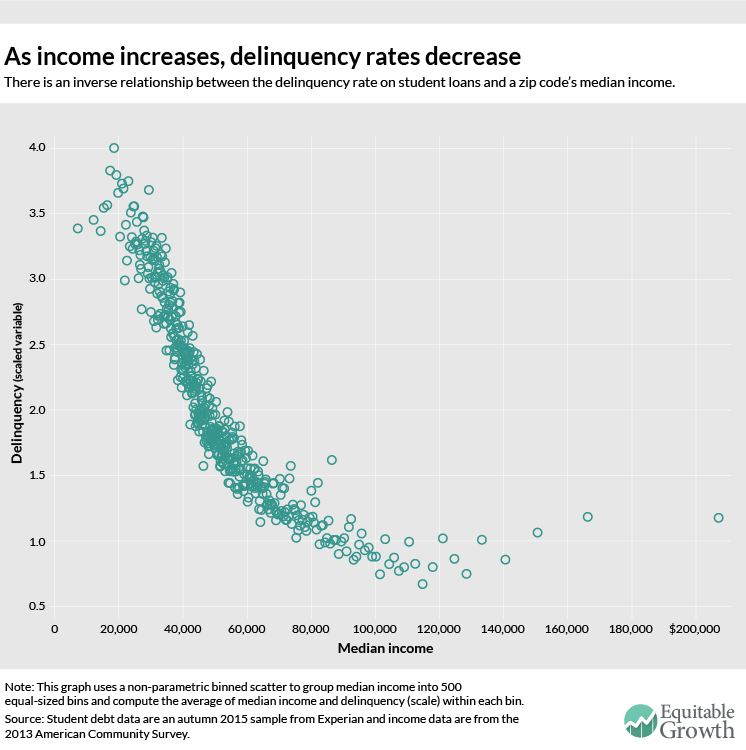
Our first Mapping Student Debt interactive released this past December revealed a striking negative relationship between income and delinquency across zip codes. Not surprisingly, we found that higher levels of income are associated with fewer problems with student loan delinquency. In this second installment of the Mapping Student Debt project, we document that the geography of delinquency is highly racialized.
Zip codes with higher shares of African Americans or Latinos show much higher delinquency. What’s more, our analysis finds that among minority student borrowers, those most adversely affected are the middle class—those who have taken out debt to go to college but who haven’t been able to find jobs or don’t have sufficient family wealth to pay it back.
Delinquency disproportionately affects minority communities
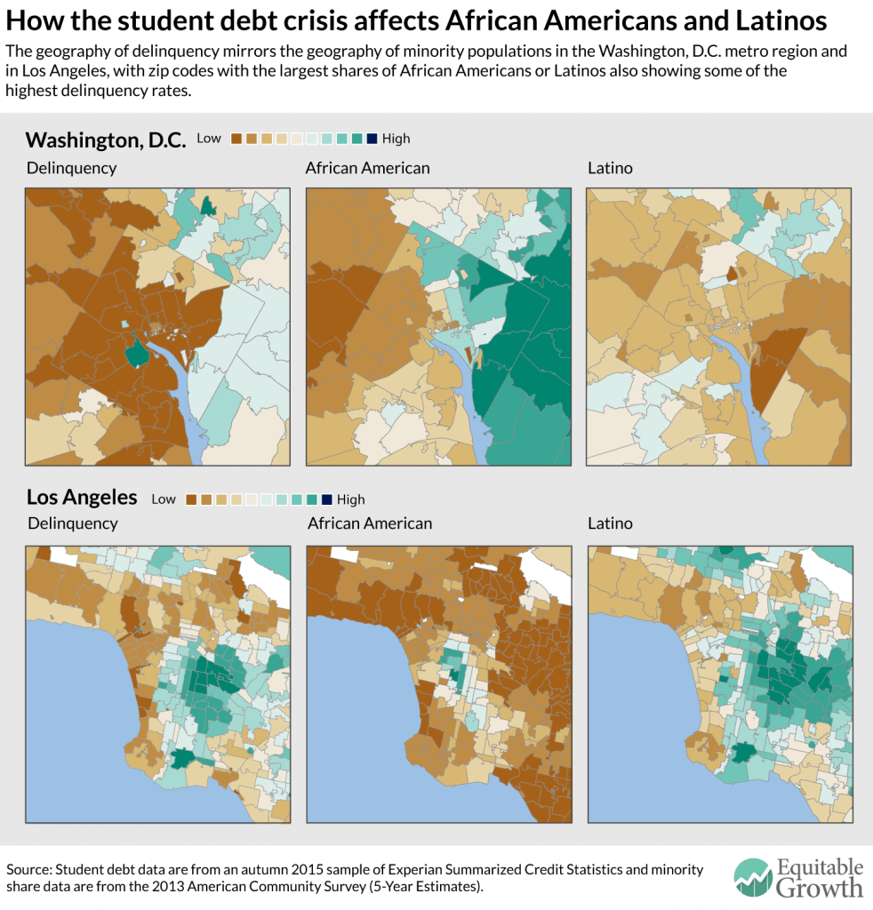
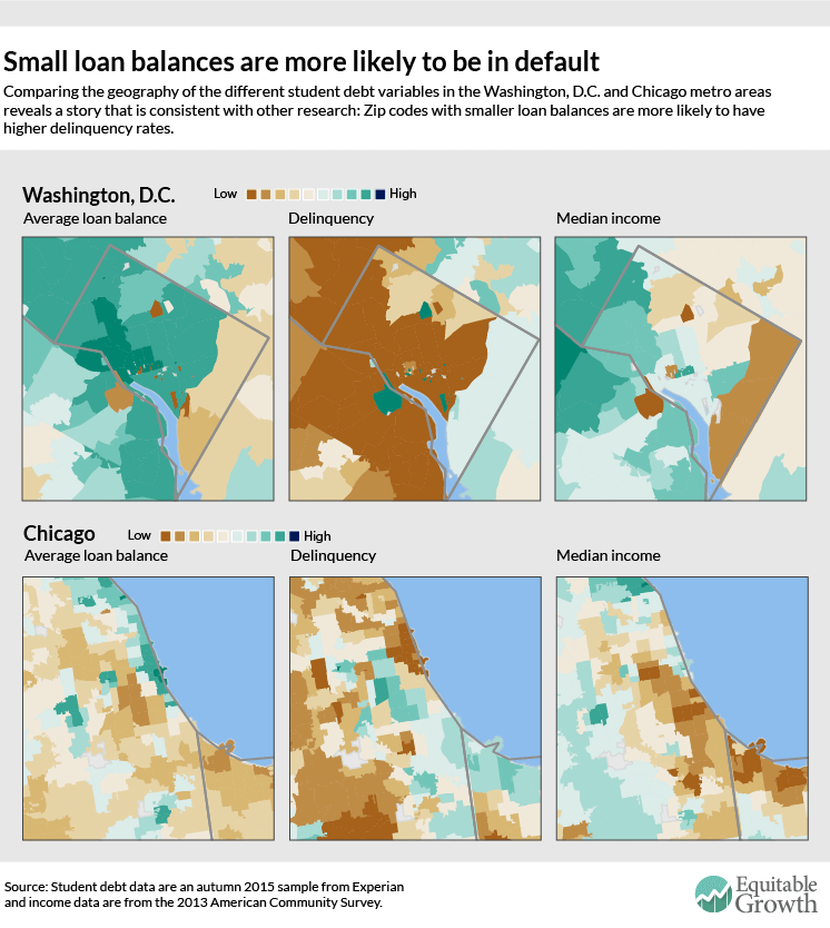
Our findings are stark. They show the strong relationship between a zip code’s minority population and its delinquency rate at both the city and national levels. In the Washington, D.C. metro region, for example, zip codes in the northeastern part of the District of Columbia and east of the Anacostia River and adjacent suburbs—all of which have the largest shares of African Americans and Latinos—also have delinquency rates that range from somewhat high to extremely high. The same pattern holds in Los Angeles, where areas with large African American or Latino populations, such as Compton, Linwood, and Huntington Park, are also where delinquency is highest. (See Figure 1.)
Figure 1
At the national level, too, we find that zip codes with higher shares of African Americans or Latinos have much higher delinquency rates. This relationship suggests that minority communities disproportionately suffer from student loan delinquency. (See Figures 2 and 3.)
Figure 2
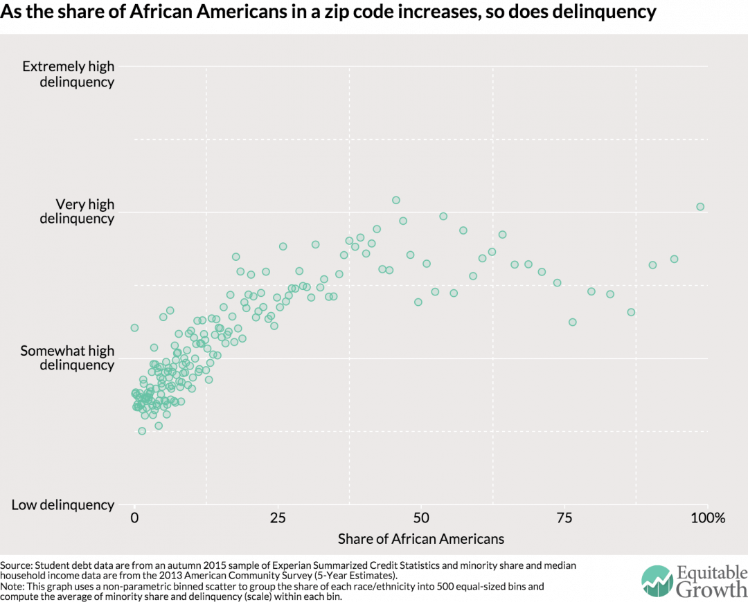
Figure 3

Controlling for income
The geography of race and of income are similar, so a natural question that arises is whether race has an independent effect on delinquency, and, if so, what is it? The answer turns out to depend on income, but not in an obvious way.
In order to investigate the effect of race independent of income, we first ranked zip codes by median income and divided them into 100 groups of equal size. Within each of these income groups, median income levels are nearly identical, which means we can look at how delinquency varies across zip codes with different shares of African Americans or Latinos but otherwise very similar income levels. In Figures 4 and 5, we plot how an increase in the minority share of the zip code population changes the rate of delinquency. Points above zero mean that as a zip code’s minority population increases (relative to zip codes with a similar income), so does the share of delinquent loans in that zip code. Conversely, a negative number implies that zip codes with larger minority populations have lower loan delinquency rates.
Figure 4
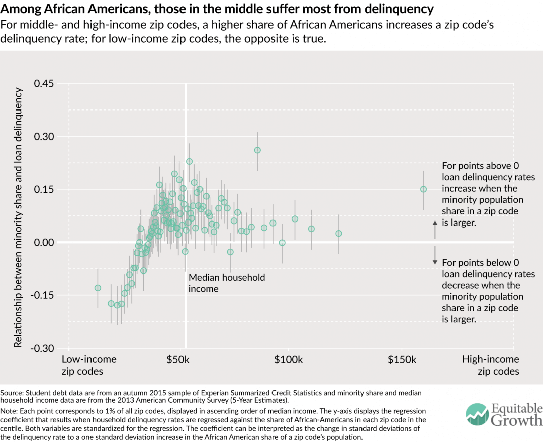
Figure 5
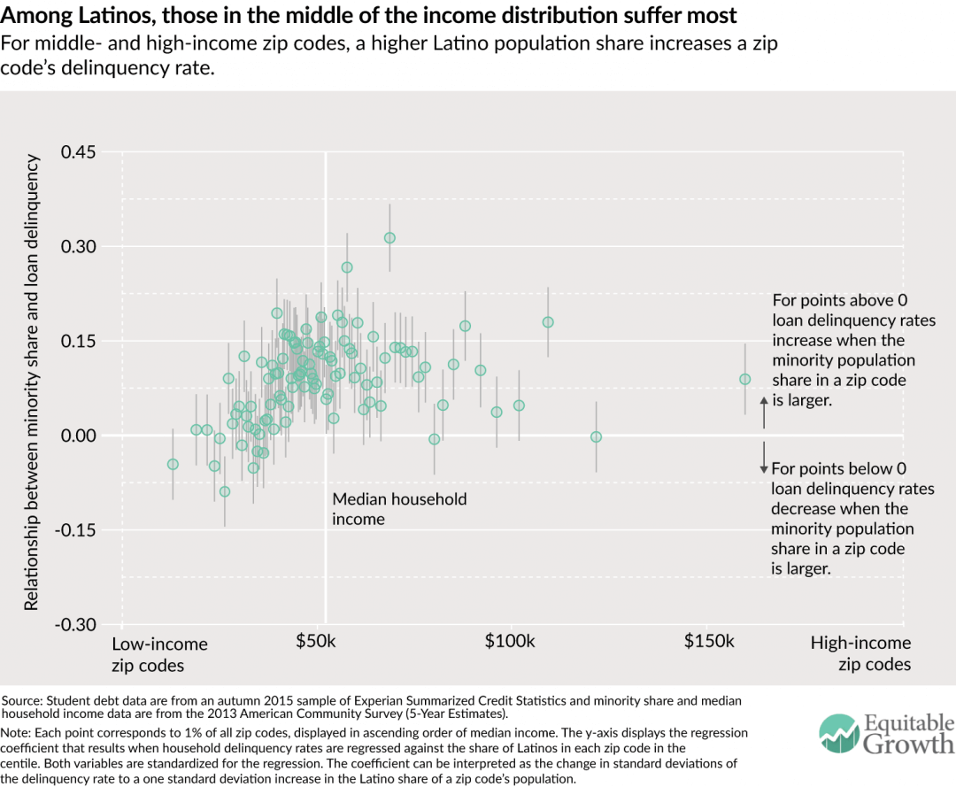
In both Figures 4 and 5, the positive correlation between the share of minorities in a zip code and loan delinquency rates is highest for the middle of the income distribution. Among zip codes with a median income of about $20,000, for example, zip codes with a large share of Latinos and those without have approximately the same rates of delinquency. But among zip codes with a median income of around $60,000, those with large Latino share have much higher rates of loan delinquency than those without.
We see a similar pattern for the share of African American in zip codes, and there the effect is even more pronounced. For zip codes with median incomes above $60,000, the effect of race on delinquency either stays roughly constant or declines slightly.
Another interesting feature of the data is that among the zip codes with the poorest populations, an increase in the share of African Americans is associated with a decline in delinquency rate, whereas the share of the Latino population has no impact on delinquency. We do not think our data are rich enough to meaningfully address this particular fact, which merits further research.
The role of race in student loan delinquency
Minority populations disproportionately suffer from high delinquency, and, within minority populations, the middle class seems most adversely affected. What can we make of these findings? We believe that these two facts reflect the impact of structural racism in the U.S. higher education system, credit and labor markets, and distribution of wealth.
African Americans and Latinos are, on average, less likely than white students to complete college once they start. According to the National Center for Education Statistics, in 2013 roughly 57 percent of recent African American high school graduates and 60 percent of recent Latino high school graduates were enrolled in college compared to 69 percent of white students. Yet the National Center for Education Statistics reports that for the 2005 starting cohort of college students, about 21 percent of African Americans and 29 percent of Hispanics complete a four-year institution within four years compared to a four-year completion rate of 42 percent for white students.
The college enrollment gap between whites and minorities is narrowing, but the college completion gap is not. One likely explanation for higher student loan delinquency among African Americans and Latinos is that the borrowing is concentrated among those who either attended for-profit or other non-traditional institutions or who dropped out—exactly the population at the margin of attending college in the first place. Furthermore, we know that higher education is racially segregated, with minorities less likely to attend—or even consider applying to—selective institutions.
Even after controlling for key risk factors, African Americans and Latinos are disproportionately served by high-cost credit providers who provide less generous terms and more onerous repayment requirements, implying that discrimination occurs through market segmentation and sorting.
Another explanation for high delinquency rates among minorities is that after college, graduates still confront significant discrimination in labor markets, with minority applicants less likely to get job offers, even after factors such as education are taken into account. Even minority students who successfully complete college suffer from higher unemployment rates and lower earnings than their white counterparts. These disadvantages extend across college majors, occupations, and the type of higher education institution that these recent graduates attended. In combination, these factors leave minority students and their families substantially more vulnerable to delinquency than comparably situated white students and their families.
A closely related issue is that, holding income constant, African American and Latino households have substantially lower levels of wealth than do white households, including financial assets that can act as a buffer against student loan delinquency in the event of job loss or some other misfortune.
Middle-class minorities are hurt the most by student loan delinquency
Why are middle-class African American and Latino students and their families the most adversely affected by student debt delinquency? The poorest minority populations generally lack access to any kind of formal credit, instead relying on payday lending and other types of informal credit access. This means that they cannot be delinquent by our measure that is based on credit reports. What’s more, they rarely go to college, so in many cases, they do not acquire student debt.
The housing crisis revealed a similar dynamic in the late 2000s. The poorest minority households lost relatively little wealth because they didn’t have any to begin with, whereas somewhat richer minority households were among the biggest losers from the Great Recession. That was because they earned enough to have bought a house under the relatively generous terms available before the housing market crash, but then they were more likely to lose their jobs and less likely to have any cushion of family wealth. It is out of these very dynamics that persistent, multi-generational racial wealth gaps are born. And it seems likely that student debt is on the same path now—a signpost of relative economic success among minorities, but also a threat. Many young people of color have gone into debt to ascend to the middle class, and been supported by their families to do so, yet it’s not having the intended effect.
These data tell us that at least with respect to longstanding group and individual income and wealth gaps between minorities and the overall population, debt-financed higher education is not the solution, and may even be contributing to the problem. The fact that, among minorities, the middle class is most strongly affected implies the problem is structural racism, not poverty. Any solution to the student debt crisis has to recognize that.
Methodology
This geographic analysis uses two primary datasets: credit reporting data on student debt from Experian and income data from the American Community Survey.
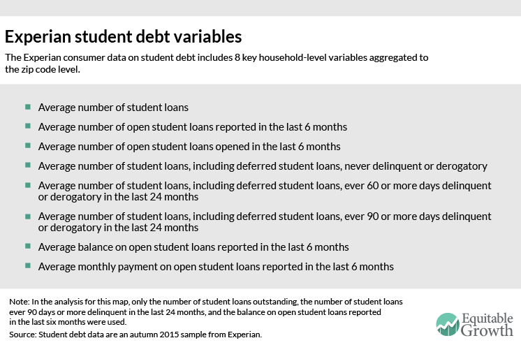
The Experian data includes eight key student debt variables (see Figure 6) aggregated from household-level microdata to the zip code level. The underlying household data are a snapshot of the entire U.S. population at a single point in time—in this case, the autumn of 2015.
Figure 6
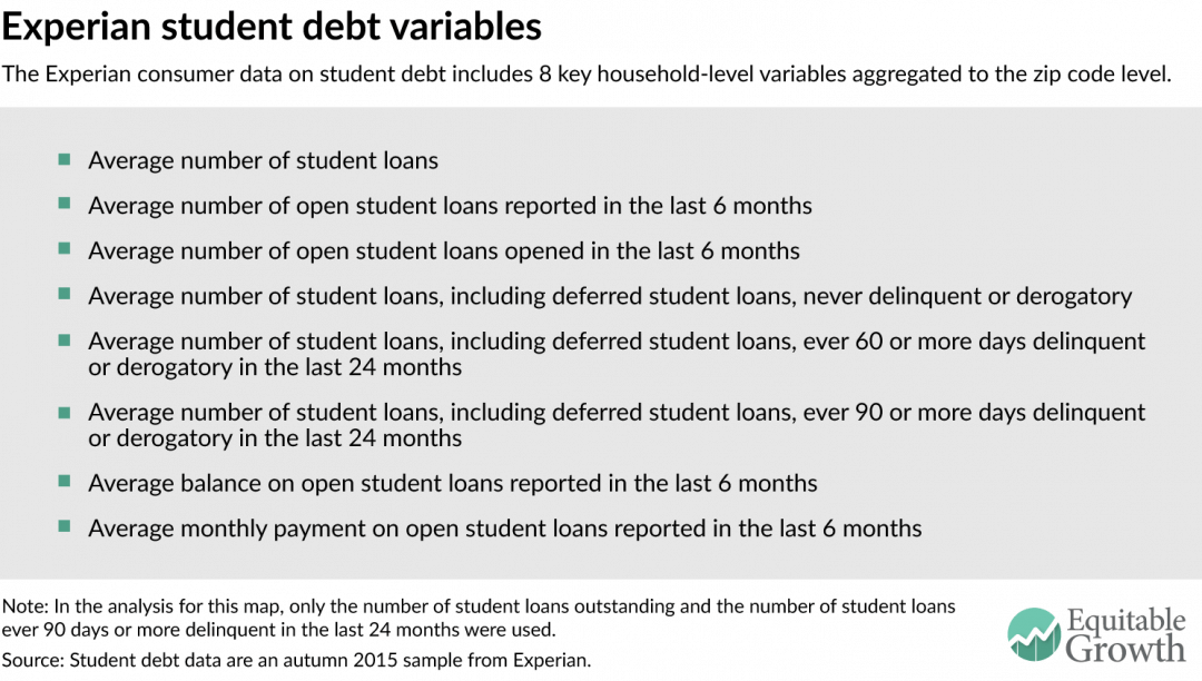
There are a number of caveats regarding the Experian data file that have guided our methodology for constructing variables and analyzing results:
- The universe of households contains only those with “any type of credit” and which, therefore, have a credit report. Relative to the population as a whole, this likely excludes the poorest households without any official credit access whatsoever.
- It is unclear how Experian constructs “households” since credit reports pertain to an individual’s credit history.
- If the same student loan has more than one signatory, then the loan may be assigned to multiple households and hence to multiple zip codes or even counted more than once within the same household.
- Experian claims that the universe of their geographically-aggregated data is all households with credit, but the levels of the data on loan balance and delinquency are more consistent with the idea that the universe is only households that have student loans. In other words, Experian claims their data include households that have credit but no outstanding student loans, but if that is the case the reported levels for average delinquency are much higher than other sources would suggest. Average delinquency rates, however, are comparable to reliable outside estimates if interpreted as delinquency among only those households with student debt.
For these reasons, we do not report any student loan data in rate amounts. Instead, we have used the Experian variable to construct an analog to relative delinquency.
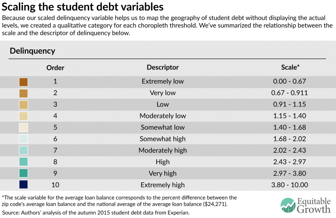
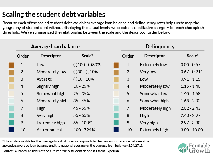
To create the delinquency variable, we calculate a “delinquency rate” for each zip code by dividing the average number of student loans that are delinquent by 90 or more days per household by the average number of outstanding loans per household. Then, after winsorizing the top 1 percent of observations to the 99th percentile value, we project the “delinquency rate” onto a scale that ranges from 0 to 10.
For user-friendliness, we assign the student debt scale variable a qualitative category. If the delinquency reads “very low,” for example, it corresponds to a scale level between 0.067 and 0.091. Figure 7 summarizes the relationship between the delinquency scale variable’s levels and its qualitative descriptions.
Figure 7
Next, we merge zip code-level household median income with data from the 2013 American Community Survey on the share of African Americans and Latinos in those zip codes along with our imputed scaled delinquency variable in order to construct choropleth maps.
The actual map uses two different techniques to display the variables on a choropleth scale. For delinquency, we created 10 quantiles (or equal counts) to account for the right-skewed data. And for the two minority share variables, we used 10 jenks (or natural breaks in the data) to assign the color scale. Higher numbers and darker shading correspond to higher shares of outstanding loans that are delinquent by 90 or more days in the previous 24 months and higher shares of African Americans and Latinos in a zip code.
Additional reading
Adam Looney and Constantine Yannelis, “A crisis in student loans? How changes in the characteristics of borrowers and in the institutions they attended contributed to rising loan defaults.”
Benjamin Backes, Harry J. Holzer, and Erin Dunlop Velez, “Is It Worth It? Postsecondary Education and Labor Market Outcomes for the Disadvantaged.”
Caroline M. Hoxby and Sarah Turner, “What High-Achieving Low-Income Students Know about College,” American Economic Review.
Devah Pager, Bruce Western, and Bart Bonikowski, “Discrimination in a Low-Wage Labor Market: A Field Experiment.”
Fenaba R. Addo, Jason N. Houle, and Daniel Simon, “Young, Black, and (Still) in the Red: Parental Wealth, Race, and Student Loan Debt,” Race and Social Problems.
Janelle Jones and John Schmitt, “A College Degree is No Guarantee.”
Jeffrey P. Thompson and Gustavo A. Suarez, “Exploring the Racial Wealth Gap Using the Survey of Consumer Finances.”
Jess Bricker and others, “Changes in U.S. Family Finances from 2010 to 2013: Evidence from the Survey of Consumer Finances.”
John Schmitt and Heather Boushey, “The College Conundrum: Why the Benefits of a College Education May Not Be So Clear, Especially to Men.”
Joshua Angrist, David Autor, Sally Hudson, and Amanda Pallais, “Leveling Up: Early Results from a Randomized Evaluation of Post-Secondary Aid.”
Martha J. Bailey and Susan M. Dynarski, “Gains and Gaps: Changing Inequality in U.S. College Entry and Completion.”
Marianne Bertrand and Sendhil Mullainathan, “Are Emily and Greg More Employable Than Lakisha and Jamal? A Field Experiment on Labor Market Discrimination.”
Neil Bhutta, Paige Marta Skiba, and Jeremy Tobacman, “Payday Loan Choices and Consequences.”
Patrick Bayer, Fernando Ferreira, and Stephen L. Ross, “Race, Ethnicity and High-Cost Mortgage Lending.”
Rakesh Kochhar and Richard Fry, “Wealth inequality has widened along racial, ethnic lines since end of Great Recession.”
Stephanie Chapman, “Student Loans and the Labor Market: Evidence from Merit Aid Programs.”
 Today, Equitable Growth kicks off “Equitable Growth in Conversation”—a recurring series where we’ll talk with economists and other social scientists to help us better understand whether and how economic inequality affects economic growth and stability in particular ways.
