Key takeaways

• Federal spending cuts slow U.S. economic growth and raise unemployment. Reductions in federal spending—whether through cuts to direct government consumption, investment, or transfer programs—consistently lower U.S. Gross Domestic Product, reduce employment, and increase the unemployment rate. The negative effects are particularly severe if the Federal Reserve is unable to offset the cuts by lowering interest rates, such as during a recession.
• The broader economic context of austerity is crucial to understanding its effects. The impact of spending cuts depends on the type of spending reduced and the Fed’s ability to respond. Cuts to federal consumption and investment have a larger and immediate negative effect on GDP than cuts to government transfer programs. When the Fed has room to cut interest rates in response to austerity, it can partially mitigate the damage, but if it is constrained—such as by the zero lower bound during a recession—the economic harm ends up being much greater.
• Austerity can be counterproductive to debt reduction. While austerity is often implemented to lower the debt-to-GDP ratio, cuts can actually increase debt burdens if they significantly shrink the economy, especially when the Fed cannot respond. This is because reductions in GDP erode the tax base, undermining the intended fiscal improvements of austerity.
• Austerity case studies show mixed results and social costs. International examples—including Thatcherism in the United Kingdom, New Zealand’s Rogernomics, Canada’s Program Review, and Greece’s debt crisis—demonstrate that while austerity can reduce deficits, it often leads to increased unemployment, reduced public services, and significant social hardship. In some cases, the economic and health consequences were severe and long-lasting.
• Layoffs have persistent negative effects on workers. Mass layoffs, such as those resulting from austerity-driven public-sector cuts, lead to long-term earnings losses (15 percent to 25 percent lower wages for up to 15 years post-layoff), higher unemployment durations, and even increased mortality risk for affected workers. The impact is more pronounced during economic downturns and for vulnerable groups, such as women and older workers.
• Policy uncertainty further depresses economic activity. Elevated policy uncertainty—often accompanying fiscal consolidation—reduces business investment, hiring, and overall economic output. This uncertainty amplifies the negative effects of austerity by discouraging economic activity and slowing recovery.

Overview

With the passage into law of the Republican budget reconciliation bill last month and the recent work of the Department of Government Efficiency under Elon Musk,¹ austerity is once again top-of-mind in federal policymaking. This report answers some common questions about austerity—what it is, its history in the United States and in other advanced nations, what its economic effects are, and how effective a strategy it is in achieving its goal of making the fiscal trajectory more sustainable.

What are the broader economic effects of cuts to federal spending?

Broadly speaking, cuts to federal spending slow down economic growth, reduce employment and labor force participation, raise the unemployment rate, and hurt state and local finances. They also can lower business investment depending on the specific type of federal cut and economic circumstances.

Different types of federal spending affect the U.S. economy slightly differently.

• Transfers—anti-poverty programs such as Medicaid and social insurance programs such as Medicare and Social Security—are not accounted for directly in Gross Domestic Product,² but they do affect GDP indirectly, primarily through household income and consumption. A cut to federal transfer programs lowers households’ post-tax-and-transfer income, and by extension consumption, shrinking demand and GDP in the short run.
• Federal consumption (the salaries of federal employees and costs of intermediate goods and services used to provide federal services to beneficiaries) and investment (infrastructure spending, procurement, and research and development, among others) are directly accounted for in GDP, since they represent the direct demand of the federal government for goods and services. So, a one-dollar cut to these spending categories has, as a first-order short-run effect, a one-dollar reduction in GDP—not to mention the second-order effects that may increase or decrease the overall effect.

The ultimate effect of changes in fiscal policy on economic output is called the fiscal multiplier. A multiplier of 1 signals that a one-dollar change in spending leads to a one-dollar change in output or GDP. The size of the multiplier depends on many factors, including the specific type of spending being changed, the amount of “slack” or excess capacity there is in the economy, and how reactive the Federal Reserve is.

A Federal Reserve that is highly reactive, which is common in most normal times, will change monetary policy quickly if changes in fiscal policy affect inflation and employment—in the case of austerity, for instance, it will cut interest rates in response. This blunts some of the negative economic effects of austerity, shrinking the fiscal multiplier. Yet a nonreactive Federal Reserve—which can happen when, say, austerity is attempted in the middle of a recession and the Fed has no room to cut interest rates further—will not counteract the economic damage from austerity, making the effective fiscal multiplier higher.

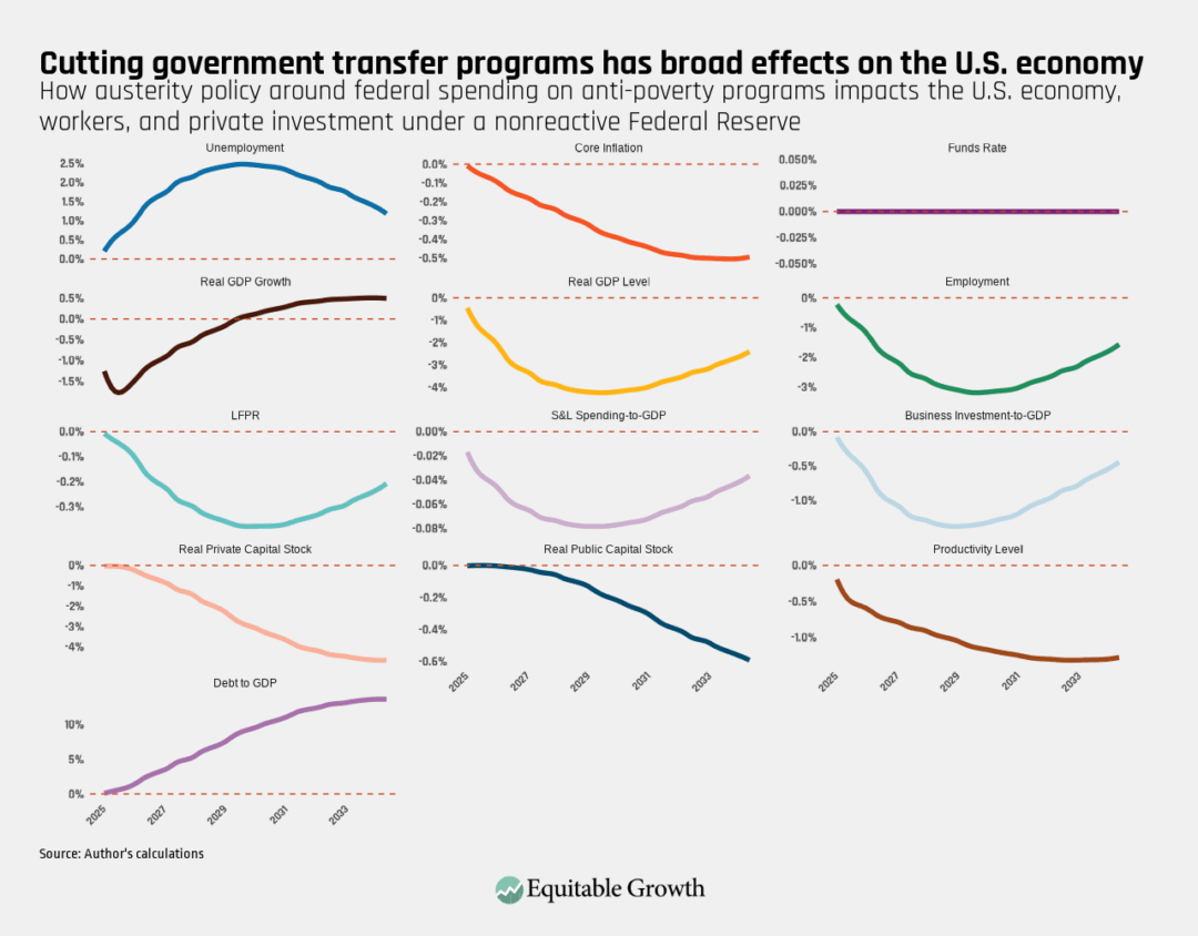
Figures 1 through 4 below use the Federal Reserve’s workhorse macroeconomic model, called FRB/US, to simulate a permanent cut of 1 percent of GDP to federal consumption and investment spending³ and, separately, to federal transfer spending under two scenarios. One is under a highly reactive Federal Reserve and one is under a nonreactive Fed that is constrained by the zero lower bound, or when short-term interest rates are at or near zero, from cutting nominal interest rates.⁴ The model shows in broad strokes what would be expected: Austerity lowers GDP and employment, raises the unemployment rate, and hurts business investment, especially in the first two years. (See Figures 1–4.)

Figure 1

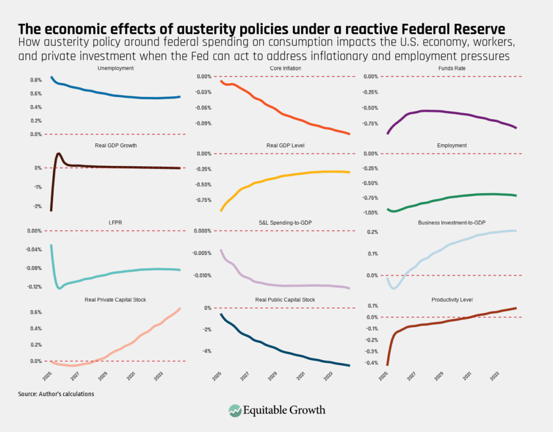
Figure 2

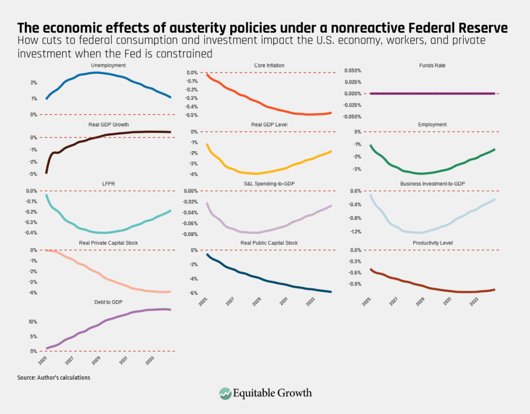
Figure 3

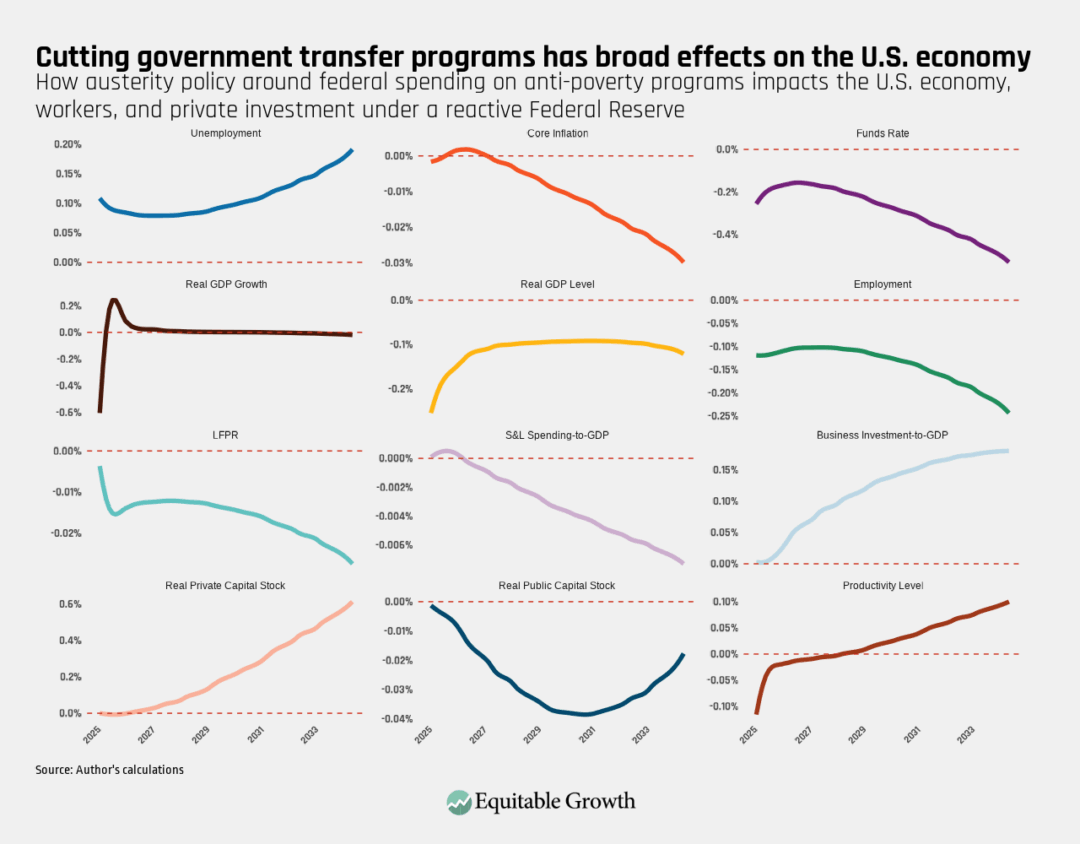
Figure 4

More specifically:

• Real GDP is lower in all four scenarios. When federal consumption is cut by 1 percent of GDP, real GDP (after accounting for inflation) immediately falls by 1 percent, regardless of the Fed’s reaction.⁵ In the reactive Fed scenario, the Fed cuts interest rates, which partially but not fully mitigates the economic weakness, and real GDP ends the decade roughly 0.4 percent smaller. When the Fed is constrained from cutting rates, the damage is worse, troughing 3 years out with GDP 4 percent smaller—or the equivalent of more than $1 trillion in lost economic activity in 2024 dollars—then ending the decade 2 percent smaller.
• A cut to federal transfer programs has a smaller but still damaging economic effect. The initial hit to real GDP from a cut of 1 percent of GDP is -0.25 percent. As with a federal consumption cut, this effect declines somewhat over time under an active Fed, ending the decade down -0.15 percent against baseline. Without Fed intervention, though, the hit is much worse, with real GDP lower by 2.5 percent at the end of the decade.
• The unemployment rate rises in all four scenarios, too. When cutting federal consumption, the effect is a consistent increase of 0.4 percentage points to the unemployment rate under an active Fed and a peak effect of an increase of 2.5 percentage points under an inactive Fed. With transfer cuts, the effect under an inactive Fed is nearly the same, while under an active Fed, the unemployment rate rises 0.1 percentage points initially and then ends the decade 0.2 percentage points higher.
• The level of employment and labor force participation rates fall. Employment levels decreasebetween 0.5 percent (under an active Fed) and 3 percent (with an inactive Fed) after a decade of consumption and investment cuts and by between 0.3 percent and 3 percent after a decade of transfer cuts. Labor force participationfalls between 0.06 percentage points and 0.4 percentage points with consumption and investment cuts and by 0.03 percentage points and 0.4 percentage points under transfer cuts.
• State and local consumption and investment spending also fall. Under federal consumption and investment cuts, part of the state and local decline in spending arises because an across-the-board federal discretionary cut will hit grants to state and local governments for priorities such as infrastructure and education. Under federal transfer cuts, the decline in state and local spending happens because of economic weakness and the adjustment of balanced-budget-constrained states to lower tax revenues. A cut of 1 percent of GDP in federal consumption and investment eventually reduces state and local consumption and investment by between 0.02 percent to 0.08 percent of GDP, while a similar decline in transfer spending reduces it by 0.01 percent to 0.08 percent of GDP.

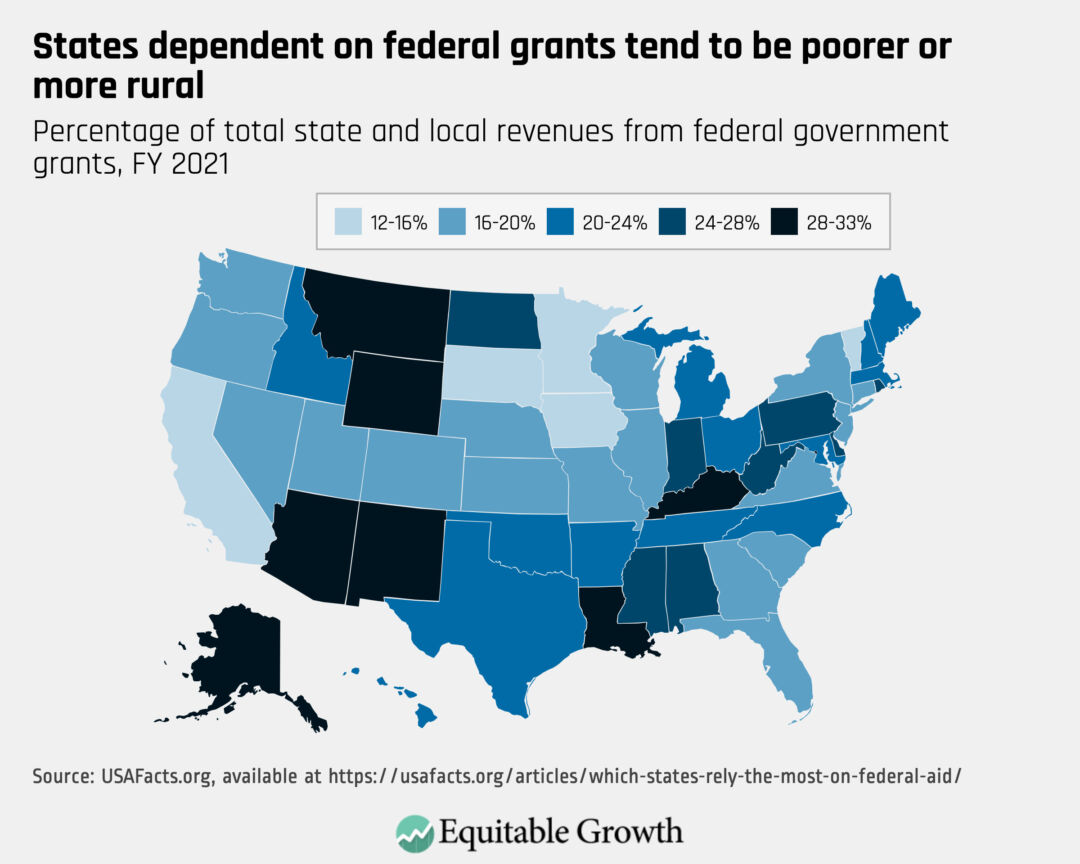
Which states get hit hardest by federal austerity? In aggregate, federal grants to state and local governments are generally correlated with population. To gauge dependence on federal grants, one can look instead at federal grants as a percent of state and local revenues. As the map below shows, the most dependent states tend to be poorer and/or more rural. Cuts to state and local aid, then, can easily fall on the most vulnerable residents.⁶ (See Figure 5.)

Figure 5

Below are several additionally telling observations from Figures 1–5:

• Private investment sees mixed results. Under the two active Fed scenarios, private investment is up by about 0.2 percent of GDP after 10 years, but it is important to note that this is mostly because the Fed is cutting interest rates to counteract the economic damage from austerity. (Some of this is also crowding-in from lower deficits and debt over time, a channel we added to FRB/US model to make sure we capture it properly.) The difference becomes evident by comparing to the inactive Fed scenarios, where real interest rates don’t decline and business investment is down by -0.25 percent to -0.4 percent of GDP after 10 years.
• The public capital stock, or the amount of government infrastructure, falls in all scenarios but much more so when federal investment is cut. This has knock-on effects that also lower state and local investment due to cuts in federal infrastructure grants. Under the consumption and investment cut scenarios, the real public capital stock is 5 percent to 6 percent smaller after 10 years, which constrains the capacity of the U.S. economy. Since a cut to federal transfers does not directly affect public investment, the fall in the public capital stock is much smaller, but it is still down by up to 0.6 percent after a decade.
• The private capital stock, or the amount of private structures, equipment, software, and R&D, differs, much like the effect on private investment itself. In the active Fed scenarios, where the central bank cuts interest rates in response to the economic weakness spurred by austerity, the private capital stock grows, somewhat but not fully offsetting the damage to economic capacity. After a decade, the real private capital stock is about 0.6 percent. Under a nonreactive Fed, the capital stock shrinks by 3 percent to 4 percent, as declines in investment compound over time.

• Private labor productivity, or the amount that workers produce each hour, falls initially in all scenarios. The rise in private investment and private capital stock under the reactive Fed scenarios leads to more labor-augmenting capital, which, over the long run, allows the level of labor productivity to recover. This doesn’t happen under a nonreactive Fed scenario, in which private investment is persistently lower, shrinking the level of productivity by roughly 1 percent after a decade.

How counterproductive is austerity in lowering the debt-to-GDP ratio?

Deficits in the United States are so high—even ignoring interest costs—that lowering the debt-to-GDP ratio requires, by definition, some combination of lower spending and higher revenues. But as our modeling shows, controlling the debt-to-GDP ratio using austerity introduces substantial counterproductive headwinds, especially if federal investment is cut and especially if the Federal Reserve is constrained by the zero lower bound, such as in the middle of a recession.

To put this in the specific context of our modeling: Without accounting for dynamic economic effects but still accounting for debt service effects, we would expect a permanent cut of 1 percent of GDP to federal spending to lower the debt-to-GDP ratio by 10 percentage points after a decade. Yet the debt-to-GDP ratio falls by only 9 percentage points after 10 years when the cuts are applied to federal consumption and investment under an active Fed, showing that the declines in GDP more than dominate the additional savings from lower interest rates. Under an inactive Fed, the story quantitatively and qualitatively flips: The debt-to-GDP ratio rises by 14 percentage points over a decade.

This finding is consistent with research that has challenged the conventional wisdom that fiscal austerity is always effective in reducing the debt-to-GDP ratio. Instead, such policies can be deeply counterproductive, particularly during economic downturns and periods of low interest rates.

Brown University economist Gauti Eggertsson’s research, for example, demonstrates that when nominal interest rates approach zero, traditional fiscal mechanics break down dramatically.⁷ The mechanism behind this counterintuitive result lies in the fiscal multiplier effect, which we described above. When governments implement austerity measures during periods of economic weakness, the resulting reduction in aggregate economic output shrinks the tax base more than the direct savings from spending cuts. This erosion of the tax base represents the endogenous component of the deficit, where fiscal policy itself undermines the government’s revenue-generating capacity.

The counterproductive nature of austerity becomes even more pronounced when examining debt-to-GDP ratios specifically. Research indicates that austerity measures can create a vicious cycle in which spending cuts simultaneously reduce GDP growth while failing to meaningfully reduce debt levels.⁸

When is austerity appropriate?

The current U.S. federal debt trajectory is unsustainable, meaning debt is growing faster than the U.S. economy in perpetuity. This mismatch between spending and revenues could eventually raise costs for U.S. families and businesses through higher interest rates, making financing, including mortgages, auto loans, and credit cards, more expensive—not to mention investment and research and development.

Note that a sustainable debt trajectory does not require a fully balanced budget. It only requires nominal debt to grow at the same rate as the economy. This can broadly be achieved through what’s known as the primary (non-interest) balance, wherein only non-interest spending is aligned with revenues—though in years where interest rates are higher than growth, a primary surplus will be necessary. In 2025, the primary balance still would have left the overall deficit at 3.2 percent of GDP.  That said, the primary balance would require substantial consolidation, as the primary deficit was 3 percent of GDP in 2025.

Austerity should be considered only reluctantly as part of the policy changes necessary to close that gap. Instead, revenue increases should be the first tool to which policymakers turn. The deterioration in the fiscal outlook since 2001—the last time the United States ran a budget surplus—was driven in significant part by tax cuts.⁹

In fact, while spending and revenues did both contribute to the extreme pivot in the debt trajectory over the past quarter century, the spending contributors often were one-time events or are now over—relief packages in the wake of the Great Recession of 2007–2009 and the COVID-19 pandemic of 2020–2023, for instance, as well as the wars in Iraq (2003–2011) and Afghanistan (2001–2021)—whereas the tax cuts passed in 2001, 2003, and 2017 have proven durable and are still weighing on lower tax receipts.

Additionally, austerity can easily backfire both distributionally (hitting the most vulnerable citizens) and economically (hitting key public investments). If U.S. policymakers must incorporate austerity into a fiscal correction, it should be paired with revenue increases and should avoid spending cuts that harm low-income Americans, children, and productive investments.

What are some historical examples of austerity from around the world?

Austerity measures—large-scale government spending cuts aimed at fiscal consolidation—have been implemented in various countries with mixed results. We now will examine the historical case studies of austerity in the United Kingdom under former Prime Minister Margaret Thatcher throughout the 1980s, New Zealand during the Rogernomics era also in the ‘80s, Canada’s Program Review in the 1990s, and the Greek debt crisis in 2010, highlighting both the fiscal outcomes and the broader economic and social effects of these policies.

But first, we turn for context to the recent DOGE cuts in 2025 in the United States.

DOGE in the United States (2025)

When President Trump took office again in January 2025, his allies began working to cut federal consumption by slashing spending, reducing staff, and shuttering agencies using the existing U.S. Department of Government Efficiency to do so (albeit in new and unprecedented ways).¹⁰ The effect of these efforts so far on federal spending is difficult to gauge, given the unreliability of numbers released by DOGE.

Overall noninterest federal spending was up 6 percent through May 2025 and up 4 percent when further excluding Medicare and Social Security—two large programs with cost adjustments whose benefits were not subject to DOGE cuts.¹¹ At the same time, federal employment in June 2025 was 62,000 jobs lower than the same month a year prior.¹²

There may be further reductions that have not yet been incorporated into labor market data. These could include delayed employment end dates, paid vacations, and the terms of buyouts, though some buyouts may have been among federal employees planning to leave anyway. Even if no new DOGE cuts are enacted, cuts so far are expected to bite harder over the course of this year and in 2026 as terminated federal employees serve out the remainder of their time and use up leave.

Thatcherism in the United Kingdom (1979–1990)

Prime Minister Margaret Thatcher’s government in the United Kingdom embarked on a program of austerity and economic liberalization during her tenure from 1979 to 1990. The UK government sought to reduce public spending as a share of GDP, primarily through the privatization of major state-owned industries, such as British Airways, British Gas, and British Telecom. Although the absolute level of government spending increased in nominal terms, its proportion of GDP fell from 44 percent to 38 percent over the decade.¹³ Notably, social security, law and order, and employment spending increased as a share of GDP, while housing and trade/industry experienced the most significant reductions.

The pace of cuts under Prime Minister Thatcher averaged about 1 percent of GDP per year, which, while substantial, was less aggressive than some other austerity programs. The British economy during this period underwent significant structural changes, with the privatized industries showing improved profit performances, according to empirical assessments.¹⁴ Yet these reforms also led to increased unemployment and greater economic inequality in the United Kingdom.

The Liverpool model, used in some studies to evaluate Thatcherism’s impact on the economy, suggests that the UK economy might have achieved more robust growth without the policy shocks introduced by austerity and rapid liberalization.¹⁵ Additionally, while the shrinking of the Public Sector Borrowing Requirement, or the amount that must be borrowed to meet budget requirements, was largely credited as the driver of reduced government spending, the overall legacy of Prime Minister Thatcher’s austerity remains debated, as many of the social costs including mass unemployment persisted beyond her tenure.

Rogernomics in New Zealand (1984–1988)

In New Zealand, the Labour government elected in 1984 included the new Finance Minister Roger Douglas, who implemented sweeping free-market reforms known as Rogernomics. The primary objective was to improve the government’s fiscal position by reducing intervention in the economy, deregulating financial markets, privatizing state assets such as New Zealand Post, Air New Zealand, and New Zealand Steel, and restructuring government departments. The reforms also included a substantial devaluation of the New Zealand dollar and the corporatization of state-owned enterprises, which had to begin operating as profit-oriented businesses.

Government expenditure as a share of GDP actually rose by 3 percentage points between 1984/85 and 1987/88, largely due to redundancy costs associated with staff reductions.¹⁶ In some cases, the severance payments exceeded short-run wage savings, demonstrating the complexity of achieving immediate fiscal savings through rapid downsizing. By 1986, 18.1 percent of New Zealanders were employed by the federal government, but this figure dropped sharply as budgets were set for each department and employment ceilings were enforced.¹⁷

Management reforms shifted public spending decisions to the local levels of government, introduced output-based budgeting, and incentivized efficiency through performance evaluations and market-based pricing of government services. While these measures increased government accountability and efficiency, they also resulted in significant job losses, particularly affecting public-sector employees.¹⁸ The social and economic disruption from these reforms led to considerable opposition, and the transition period was marked by increased unemployment and hardship for many workers.

Canada’s Program Review (1994–1996)

Canada’s Program Review, announced in the 1994 budget, aimed to eliminate a 5.5 percent GDP deficit by rigorously reviewing all federal programs for necessity, efficiency, and affordability. The process involved department managers directly, who were given strict guidelines and tasked with examining $52 billion worth of government spending. The 1995 budget sought to cut $25.3 billion from government expenditure over 3 years, with some departmental budgets halved in that period. The expected reduction in federal employment was about 45,000 jobs, or roughly 14 percent of the workforce, with some positions transferred to the private sector.¹⁹

Cost-cutting measures included early retirement incentives, cash-based departure incentives for federal employees, augmented employee-transition services, and the suspension of certain employment protections. The cost of early departure incentives alone was budgeted at $1 billion.²⁰ The cuts averaged 20 percent across departments, with some facing reductions of up to 60 percent. The reductions were implemented with little prior research, consultation, or negotiation and were largely directed by Finance Minister Paul Martin.

While the Program Review is credited with eliminating the deficit and significantly reducing the debt-to-GDP ratio in Canada, it also led to the loss of many public-sector jobs and the contraction of government services. The process was notable for its scale and speed, and for the challenges it posed to government employee morale and service delivery.²¹

Greek debt crisis (2010)

The Greek debt crisis in 2010 saw the implementation of some of the most severe austerity measures in postwar Europe, particularly in the health sector. Prior to 2008, Greek health spending was among the highest in Europe, and even after deep cuts, it remained substantial.²² Yet the scale and suddenness of the reductions were unprecedented, with public spending on pharmaceuticals dropping sharply and hospital employment declining by 15 percent by 2015 compared to 2010. Preventive care, vaccination rates, and diagnostic procedures, such as CT and MRI exams, all decreased during the crisis.

Austerity in Greece was associated with increases in the crude death rate—simply the number of deaths divided by the total population—and “amenable mortality”—or deaths that could have been avoided through good quality care—as well as a rise in low birth weights and a plateau in infant mortality rates, which had previously been declining. Disease outbreaks, including influenza and West Nile fever, became more common, and there was evidence of increased suicides and mental health issues.²³

The Greek experience underscores the risks of rapid and deep austerity in essential services, where the consequences can be immediate and severe, affecting the health and well-being of the population.

What are the long-term effects of layoffs on workers?

Layoffs can have lasting adverse effects on workers. Even when the circumstances surrounding layoffs suggest that they are not due to poor performance (as with mass layoffs arising from reorganization of a firm or the closure of an entire plant, or federal layoffs since the beginning of the second Trump administration), workers who are laid off face persistently lower earnings on average. Research based on a range of contexts suggests that average annual earnings of workers who had been stably employed but lost their jobs as part of a mass layoff are about 15 percent to 25 percent lower than they otherwise would have been, an effect that persists for 15 years or more in some settings.²⁴

Average earnings losses tend to be larger for workers laid off when macroeconomic conditions are worse.²⁵ Earnings losses also tend to be larger for women than for men and more persistent for older workers than for younger workers.²⁶ Average effects, however, mask significant heterogeneity. Some workers experience losses much larger than the average effects of mass layoffs, while others, especially those who find new jobs quickly, see little effect on their long-term earnings.²⁷

For workers who experience substantial earnings losses, the losses are driven by a combination of increased time spent not working and reduced wages.²⁸ Increased time spent out of the workforce is especially important immediately after workers are laid off, and reduced wages become more important as time goes on. Importantly, wage reductions largely reflect workers finding subsequent jobs at lower-paying firms or in lower-paying occupations rather than workers becoming less productive.²⁹

In fact, increased time out of work and reduced wages interact. When workers spend more time out of work following layoffs they tend to suffer larger earnings losses in part because they ultimately find jobs at lower-paying firms.³⁰

There also is some evidence that being laid off increases a person’s mortality risk. One study of workers in Pennsylvania found that job displacement increased death rates by 15 percent to 20 percent over the following 20 years.³¹ If this effect persists beyond that period, it translates into a 1.5-year reduction in life expectancy for a worker laid off at age 40.

How does policy uncertainty affect economic outcomes, such as investment, output, and employment?

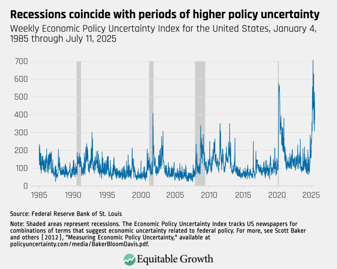
Increases in policy uncertainty adversely affect the economy by making it harder for businesses, workers, and consumers to make decisions. By one commonly used measure, the Economic Policy Uncertainty Index, which largely reflects the prevalence of uncertainty in news coverage and disagreement among economic forecasters, U.S. economic policy uncertainty reached its highest levels on record in April 2025, amid the Trump administration’s tariff announcements.³²

Research based on that measure suggests that increased uncertainty leads to reductions in aggregate measures of investment, economic output, and employment.³³ This is consistent with model-based predictions about the effects of policy uncertainty.³⁴ (See Figure 6.)

Figure 6

Research based on firm-level data also points to reductions in economic activity due to increased policy uncertainty. Studies find that policy uncertainty reduces investment, reduces hiring and increases layoffs, and makes firms less likely to pursue mergers and acquisitions.³⁵ Trade policy uncertainty, in particular, reduces investment, as well as other forms of economic activity.³⁶

---

Did you find this content informative and engaging?
Get updates and stay in tune with U.S. economic inequality and growth!

Stay updated on our latest research