Issue brief: Employers may be behind the problems with U.S. hiring

JobNewsUSA job fair in Miami Lakes, Fla.

Hiring is difficult these days. But how concerned should policymakers be? Employers in the United States are finding it more and more difficult to fill vacant jobs, as the ratio of hires-to-vacant jobs was 0.9 in January 2018, significantly lower than the average of 1.3 during the previous economic expansion of 2001 to 2007—a difference of more than 1 million newly hired workers. This decline started as the recovery from the Great Recession began—see Figure 1—but is the decline in the ratio (known as the vacancy yield) a sign of a very tight labor market, or are there other forces in the labor market that are causing a decline in the matching of open jobs to willing workers?

Download File
Employers may be behind the problems with U.S. hiring

Read the full PDF in your browser

Figure 1

A look at the data on vacant jobs and hiring shows more nuanced developments. The decline of the vacancy yield has been driven by the recovering labor market because the yield is declining as unemployment falls as well. But the vacancy yield has fallen much faster than previous experience would have predicted. Employers are increasingly reticent to hire workers already with a job—a development that is much different from the prevailing explanation that unemployed workers or workers outside of the labor force could not get hired again. In fact, the hiring of workers without jobs is in line with the current strength of the labor market.

The future path of the vacancy yield may continue to decline because the labor market ratio of unemployed workers-to-vacant jobs consistent with strong and sustainable wage growth appears to have declined. To simplify things a bit, employers could be finding it harder to hire new workers because the labor market is getting tighter; workers may be less willing to take jobs; employers may be less willing to increase wages to hire workers; or it could be some combination of the three.

If the decline in the vacancy yield is due entirely to a tightening labor market, then employer complaints about hiring would be mostly a complaint about a labor market heading toward full employment. Employers have a relatively easier time hiring workers when the labor market is weak. They have to spend fewer resources searching, as there are so many workers actively looking for work who will come to the employers. A larger supply of unemployed workers also reduces the bargaining power for each worker, pushing down the starting wage, all things being equal. Both factors make the cost of hiring a worker when the labor market is slack relatively cheap.

Graphing the vacancy yield against a measure of labor market tightness such as the ratio of unemployed workers-to-job openings would be a quick check of the validity of this cyclical development. A higher ratio indicates a weak labor market with many more unemployed workers per available job, and a lower ratio signals a tighter labor market. Figure 2 uses data from the Job Openings and Labor Turnover Survey, or JOLTS, from January 2001 to December 2017 to show that the decline in the job vacancy yield doesn’t appear to simply be the result of a tightening labor market.

Figure 2

The data show that the vacancy yield has declined as the labor market tightened, but the decline has been much stronger than just the health of the labor market would have predicted. If the relationship between the vacancy yield and the unemployment ratio from 2001 to 2007 still held, then there would have been roughly 1.1 hires per vacancy in January 2018. Instead, there were only 0.9. That might seem like a small difference, but with 6.3 million job vacancies in January 2018, an increase of 0.2 hires per vacancy would have resulted in 1.2 million more workers hired.

The difficulty in filling jobs is not simply a cyclical phenomenon but may be caused by a change in the “matching efficiency” of employers and employees. Something has changed the rate, given the health of the economy, at which vacant jobs and workers match to create a new hire. One way to see if there’s been a structural change in unemployed workers getting jobs is looking at the Beveridge Curve, which details what the unemployment rate will be for a given amount of job vacancies posted by employers.

Consider the unemployment rate as a measure of labor supply and the vacancy rate as a measure of labor demand. The data on job vacancies come from the Job Openings and Labor Turnover Survey, a U.S. Bureau of Labor Statistics dataset. When the vacancy rate declines—employers are posting fewer jobs—the unemployment rate will increase, as more workers are losing jobs and fewer unemployed workers flow into employment. When employers post more jobs and the vacancy rate increases, the unemployment rate will decline, as more workers flow out of unemployment. The result is that the Beveridge Curve is a downwardly sloping line when the unemployment rate is on the horizontal axis, and the vacancy rate is on the vertical axis. (See Figure 3.)

Figure 3

The current relationship between unemployment and job vacancies appears to be consistent with the curve before the Great Recession of 2007–2009, despite a winding road back. Therefore, a decline in the hiring of unemployed workers is not a candidate for explaining the shift in the vacancy yield.

But if the Beveridge Curve indicates that unemployed workers can just as readily get hired for jobs as in the past, then what explains the structural decline in the vacancy yield? The key distinction here is that newly hired workers who were previously unemployed are only a subset of all hiring. Not all hiring is the result of unemployed workers gaining jobs. New hires also include workers who previously had a job and jobless workers from outside the labor force who don’t register as officially unemployed. The decline in hiring might be broad-based across all these types of new hires or concentrated in one group. Understanding where new hiring declined the most may be helpful in diagnosing the cause.

Unfortunately, the data on hiring in JOLTS do not let economists look at workers’ previous employment situation before they were hired for their new job. Yet there are ways to disaggregate hires using other datasets in order to see what kinds of workers are finding new jobs. In a working paper, economists Peter Diamond at the Massachusetts Institute of Technology and Ayşegül Şahin at the Federal Reserve Bank of New York use data from the Current Population Survey to break out newly hired workers according to whether they were previously unemployed, employed, or previously not in the labor force.1

Their results are quite stark. New hires not previously in the labor force during the current recovery are in line with previous recoveries. New hires from the ranks of the unemployed are a bit out of line with previous recoveries, but their data cover only up to the first quarter of 2016. But using the same dataset as Diamond and Sahin, Figure 4 shows that new hires from unemployment are roughly in line with previous recoveries.

Figure 4

But the set of newly hired workers that’s clearly declined is new hires from employment, or job-to-job moves. As the U.S. labor market has tightened, employers are making fewer hires from workers already employed at other firms than during the past recovery. This decline is not just a product of the current recovery. The response of job-to-job hires to labor market tightness during the 2001–2007 recovery was weaker than during the economic recovery before it (from 1991 to 2001), according to Diamond and Sahin’s data. In other words, the structural decline in job-to-job moves is an almost 17-year trend.

What’s behind the decline in the matching efficiency of new hires for already-employed workers? If employers really want to fill vacant jobs with already-employed workers, then the onus is on them—employers need to increase wages in a bid to poach new employees from among the already employed. That development would be evident in the data on wages and wage growth for workers if wages and wage growth were increasing quite a bit as employers fill vacancies. Yet the data on the wage growth experienced by job switchers show the exact opposite.

The Wage Growth Tracker from the Federal Reserve Bank of Atlanta shows the long-term decline in median wage growth for workers who switch jobs. Median wage growth increases as the labor market tightens, but the peak during each subsequent recovery has been lower than the previous high.2 (See Figure 5.)

Figure 5

This trend indicates that employers are failing to increase wages or boost wage growth to fill vacancies, which, in turn, is indicative of a decline in matching efficiency on the employer side. Employers may seemingly want to hire but aren’t willing or able to pay the wages to do so. In contrast to complaints about the quality of available workers—the so-called skills gap3—the decline in matching of already-employed workers appears to be driven by changes on the employer side of the bargaining table. Exactly why companies are less willing or able to raise wages in order to poach workers deserves attention from both researchers and policymakers. Jobs aren’t getting filled, and the tightening labor market isn’t entirely behind this situation.

How much lower will the vacancy yield fall?

Given the structural forces pushing down the vacancy yield and an unemployment-to-vacancy ratio near historic lows, has the vacancy yield gotten as low as it can? Put another way: Is the historically low vacancy yield an indication that the U.S. labor market is at full employment? At first blush, there is reason to be skeptical of that claim, given the restrained rate of wage growth in recent years. Other indicators such as the prime-age employment (ages 25 to 54) rate point toward continued labor market slack.4 But returning to the Beveridge Curve, there is some more evidence that the labor market can continue to tighten.

The Beveridge Curve appears to be back in line with its pre-recession trend, which would mean that the unemployment rate for a given job vacancy rate hasn’t changed. Yet there’s also the possibility that the vacancy rate for a given unemployment rate has changed. This relationship is described by the job creation curve, which captures employers’ decisions to post a job vacancy for a given amount of labor supply. When the labor market is weak and there are many unemployed workers, the cost of filling a job is quite low and employers post more vacancies. When the labor market is tight and finding workers is difficult, the cost of filling a job is higher and fewer vacancies will be posted. The job creation curve is therefore upward sloping when the unemployment rate is on the horizontal axis, and the vacancy rate is on the vertical axis. (See Figure 6)

Figure 6

Another way to describe the job creation curve is that employers post more vacancies when they have more bargaining power and post fewer vacancies when they have less power. The economy moves along that line over the course of a business cycle, but structural shifts in the bargaining power of employers or employees could shift the whole line. An increase in worker bargaining power, for example, would shift it down and to the right, while more powerful employers would shift the curve up and to the left.

Economists Andrew Figura and David Ratner at the Federal Reserve Board argue that a structural tilt in bargaining power toward employers has shifted the job creation curve.5 They look at the relationship between the labor share of income—a proxy for employee bargaining power—and the ratio of job vacancies-to-unemployed workers. If the decline in the labor share of income is due to increased employer power, then industries and states that experienced larger declines in labor’s share of income will see a larger increase in the number of vacancies per unemployed worker.

Figura and Ratner find just such relationships in the data and argue this implies the job creation curve has shifted such that today, employers will post more vacancies for a given unemployment rate. With an unchanged Beveridge Curve, a shift in the job creation curve would mean a lower equilibrium unemployment rate, a higher equilibrium job vacancy rate, and a lower equilibrium unemployment-to-vacancy ratio. All three developments would be consistent with a U.S. labor market that has room to run.

If the U.S. labor market is really at this new equilibrium, then the current job vacancy rate might be low by historical levels but still not low enough to be consistent with full employment. The labor market looks to move further down and to the left on Figure 2, which would lead to a continued decline in the vacancy yield. It’s unclear how much further it could go—and it won’t become apparent until wage growth starts to pick up significantly.

Conclusion

The decline in the rate at which vacant jobs posted by employers are turning into hiring of new workers is one part encouraging and one part concerning. The declining vacancy yield is consistent with a tightening labor market. Furthermore, unemployed workers and workers outside of the labor force don’t appear less likely to be hired given the state of the labor market. Yet employers seem less willing to raise wages in order to poach other companies’ employees.

For policymakers, these results have three implications. The first is that the historically low vacancy yield does not necessarily mean the labor market is at full employment. Employers seem more willing to post job vacancies than in the past, meaning the yield can fall much lower without significantly pushing up wage growth. Increasing employer complaints about the difficulty of hiring may be the price of getting the labor market all the way to full employment and strong wage growth.

Secondly, a tighter labor market may not boost the bargaining power of workers as much as in the past. A higher vacancy yield for a given level of labor market tightness tilts the bargaining table toward employers. Policymakers interested in boosting workers’ bargaining power should be aware that structural reforms need to be made in addition to hitting the cyclical goal of full employment.

Finally, employer complaints about being unable to find workers to fill jobs should be taken with a grain of salt. The fact that workers are flowing out of unemployment at rates consistent with past experience in combination with relatively tepid wage growth is an indication that a viable labor supply is available, just perhaps not at the price employers would like to pay in wages. A deeper understanding of the origins of employers’ hesitation to boost wages to poach talent should inform policymakers’ efforts to increase hiring among already-employed workers.


The evolution of charter school quality in Texas

A KIPP charter school student holds up a practice test during class in Houston.

Charter schools are an increasingly popular alternative to traditional public schools for families across the United States. Charter schools were initially hailed as sources of educational innovation and as facilitators of school choice because they brought market mechanisms into educational markets. But after the rapid expansion of the charter sector over the past two decades, these schools remain controversial. The reason stems in part from the mixed empirical evidence of the effectiveness of charters at raising student achievement. On the one hand, lottery studies focused on specific oversubscribed urban schools generally find positive effects among students who attend charter schools. But on the other, studies using a broader set of schools tend to find smaller or even negative impacts on student achievement.

The problem with both sets of studies is that they generally evaluate schools at one point in time, which tells educators and policymakers alike relatively little about the overall performance of the charter school sector. Evaluating the market-oriented reforms that were originally explicit in the charter movement requires examining the dynamics of their educational achievement over time. In our working paper “The Evolution of Charter School Quality,” my co-authors and I study these charter school sectoral dynamics using longitudinal microdata on students and schools made available by Texas Schools Project, a research institution interested in educational policy questions. These data allow us to characterize the full distribution of school quality as measured by school-level value added for both charter schools and traditional public schools.

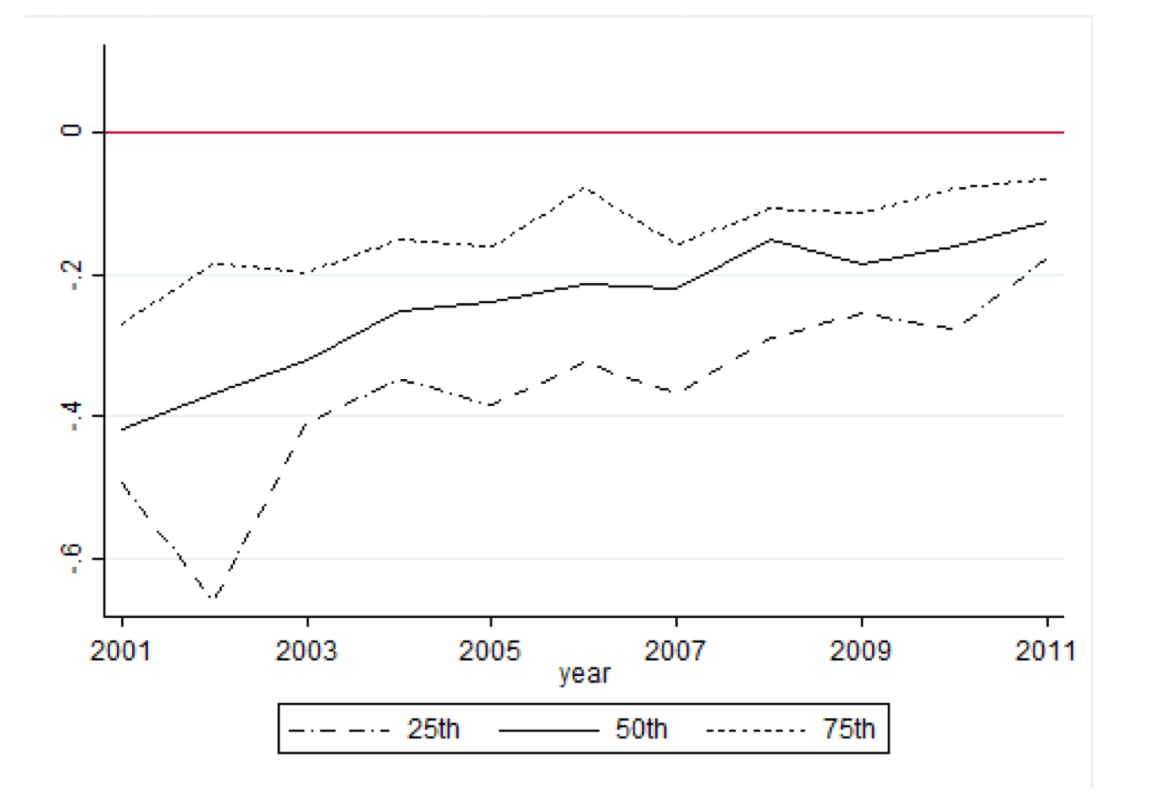
Figure 1 below presents the 25th, 50th, and 75th percentiles of the distribution of school effectiveness in mathematics for charter schools relative to the corresponding percentiles for their traditional public school counterparts. The figure highlights the steady improvement of charter schools relative to traditional public schools in Texas between 2001 and 2014. Using our preferred model (see our working paper), we observed substantial improvement in charter school value—roughly 0.25 standard deviations in math and 0.22 standard deviations in reading at the mean.

Figure 1
The improving relative performance of charter schools versus traditional public school in Texas
Charter school educational quality over time relative to traditional public schools in mathematics, 2001–2014
<em>Note: Figures show the difference between the 25th, 50th, and 75th percentiles of the charter and traditional public school quality distributions based on statewide value-added models.<br />Source: Authors’ calculations from Texas Schools Project microdata</em>

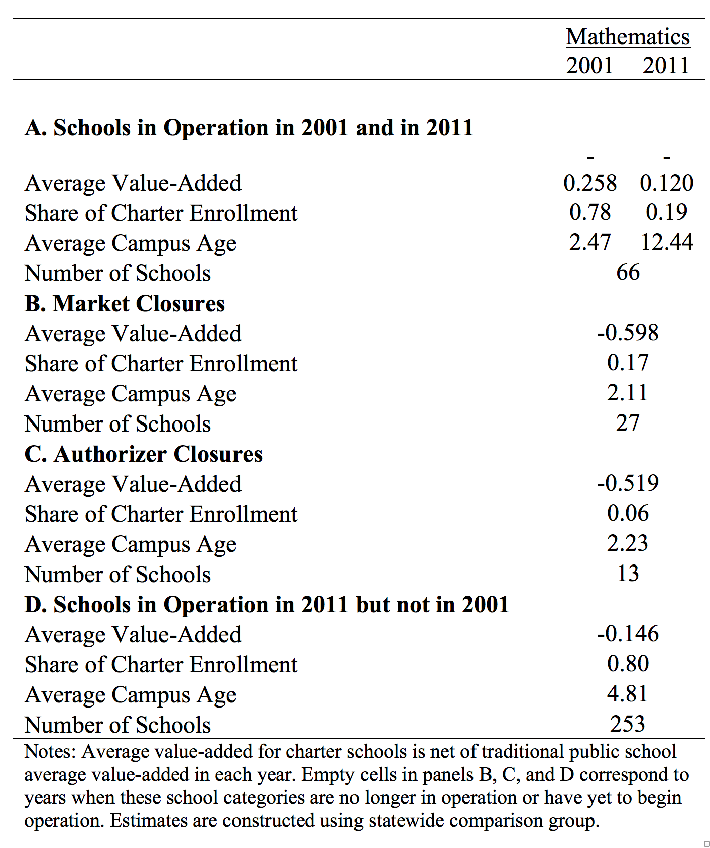
My co-authors and I next examine how the dynamics of charter schools’ entry, exit, and persistence in the educational marketplace in Texas drives the evolution of school quality. We observe three features of these dynamics that are consistent with market forces. First, the schools that closed either voluntarily or by the Texas Education Agency were, on average, the worst performers. Among schools that were open over the entire period, there was improvement in mathematics relative to their traditional public school counterparts. (See Table 1.)

Table 1
Charter schools that closed were typically the worst performers
Average value-added, enrollment, and length of operations of charter schools in mathematics for 2001 and 2011, by status of school operations
<em>Source: Authors’ calculations from Texas Schools Project microdata.</em>

Finally, among the charter schools that were new entrants, their performance, on average, was much closer to those that persisted in the marketplace compared to those that closed. This last finding probably reflects that during the period we study, most new charter schools in Texas were due to expansion within so-called charter management organizations, or CMOs, which oversee the rollout of new schools and overall operations of the system. These results suggest that relatively successful CMOs may be, in many cases, figuring out what works in their schools and replicating it.

We then look deeper into three possible sources of this observed improvement considered in the educational literature on school:

  • Reductions in school turnover
  • Increases in the share of charter schools that adhere to a “no excuses” educational philosophy
  • Pre-enrollment differences among charter school enrollees

In the paper, we first present evidence that the number of new schools accelerated in the latter part of our observation period, yet the fraction of students attending new schools declined steadily over the period. This suggests that charter schools are maturing as a sector over time.

Second, and consistent with existing literature that points to the relative success of the “no excuses” style curriculum in a number of settings, we find that the improvement of charter schools in Texas has coincided with such schools capturing an increasing share of the charter school market. Several important studies report evidence of the strong performance among charter schools that set high expectations, required uniforms, or more broadly adopt a “no excuses” philosophy, among them a 2012 study published by Mathematica Policy Research, a 2013 study by Joshua Angrist and Parag Pathak at the Massachusetts Institute of Technology and Christopher Walters at the University of California, Berkeley, and another study that same year by Will Dobbie of Princeton University and Roland Fryer of Harvard University.

Third, we present evidence of changes over time in the composition of who attends charter schools. Our results suggest that, in comparison to demographically similar students who attended the traditional public schools from which these charter school students were selected, these new charter-school students are increasingly positively selected on the basis of their pre-charter achievement scores, as well as a lower likelihood of having a disciplinary infraction in the previous year. Moreover, in comparing students who remained at the charter school with students who left after a year, we find evidence again that those students who remained exhibited higher pre-charter enrollment scores.

Importantly, regression evidence reported in the paper shows that including controls for increasing positive selection of charter school student entrants and reductions in student turnover does not mitigate the robust positive relationship between charter school effectiveness and adopting a “no excuses” curriculum. In short, the curriculum and disciplinary structure of the school seem to be a key part of improving charter school quality.

Notwithstanding the suggestiveness of these findings, these potential sources of improvement explain only a fraction of the improvement in the effectiveness of charter schools. The findings suggest the value of taking a longer-term perspective when evaluating the impact of a major educational reform such as the introduction of charter schools, especially when the success of the reform ostensibly depends on parental decisions and market forces. But the findings also point to the necessity of further research on the role of principals and other aspects of school operations, as well as the behavior of families with children attending charter schools in leading to better educational outcomes for those students.

—Marcus Casey is an assistant professor of economics at the University of Illinois at Chicago and the David M. Rubenstein Fellow at the Brookings Institution.

Factsheet: Gender wage inequality in the United States and what to do about it

Over the past 40 years, women in the United States increased their work hours, and their rising incomes became a significant part of overall household financial stability. More working women also contributed mightily to stronger economic growth. These additional earnings have made the financial difference for families across races and up and down the income spectrum while also boosting economic growth.

Download File
Fact sheet: Gender wage inequality in the United States

Read the full PDF in your browser

Yet despite all of these gains, women are still severely limited by gender pay inequality, which for a number of reasons keeps women’s average earnings at nearly 20 percent less than men’s average earnings. Here are the topline numbers from the Washington Center for Equitable Growth’s new report, “Gender wage inequality: What we know and how we can fix it.”

  • Women make up half of the U.S. population (50.8 percent)6 and are close to half of all currently employed workers (46.7 percent).7
  • The average earnings of all women who work full time, year round is 80.5 percent (routinely reported as 81 percent) of men who work full time, year round.8 This adds up to total wage differences of more than $799 billion annually.
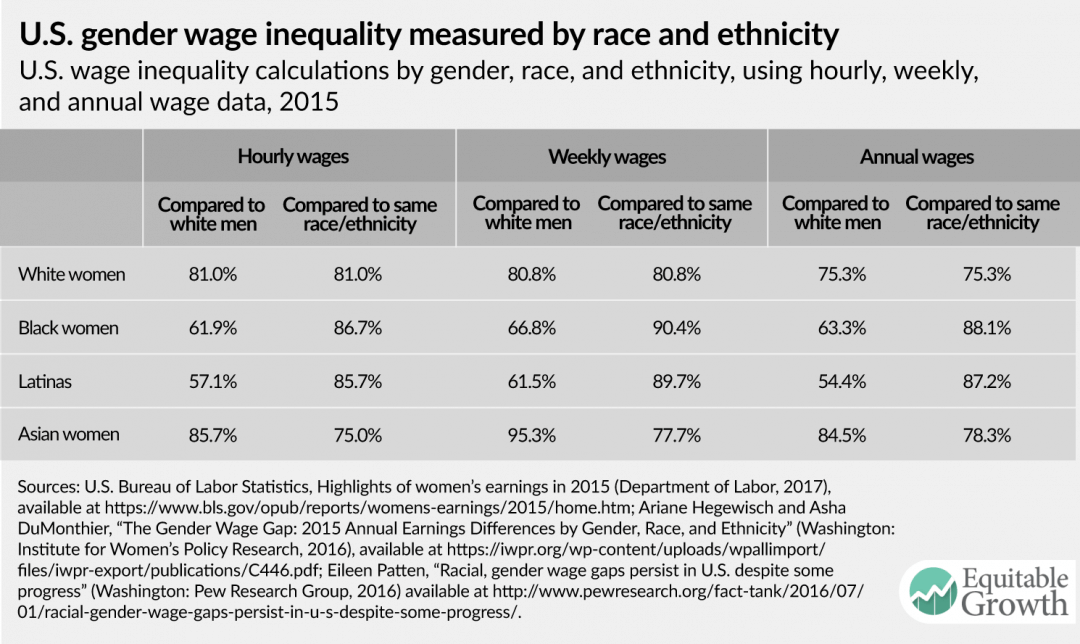
  • The wage gap is worse for black women and Latinas. (See Table 1.)
  • Table 1

  • Women’s earnings are critical to families’ financial well-being. Women are more likely than men to be single heads of households raising children. And as wages have stagnated, the families that have experienced real, inflation-adjusted income growth since the 1970s are likely to be married couples where the wife works.9
  • Women’s earnings also support economic growth. Research finds that if women had not increased their work hours since 1979, GDP in 2012 would have been 11 percent lower than it would have been otherwise, resulting in $1.7 trillion less in output.10

What are the causes of gender pay inequality, and what can we do about them?

Work experience

Women have less work experience than men, which explains 14 percent of gender wage inequality—resulting in $112.7 billion in lost wages annually. Gender differences in work experience are largely because women are more likely than men to cut back their work hours or drop out of the labor force altogether due to family and other outside obligations.11 Women are also more likely than men to be part-time workers, who receive lower hourly wages and fewer benefits compared to those doing the same job full-time regardless of gender.12

Policies that make it easier for women and men to be both workers and family caregivers such as paid family and medical leave and public support for universal childcare can help increase women’s work experience by allowing them to remain connected to the labor force.

Industry and occupation

Just more than half of gender pay inequality—50.5 percent—can be explained due to gender differences in the industries (17.6 percent) and occupations (32.9 percent) where men and women work, amounting to a combined estimate of about $404 billion dollars in wage differences. Wages tend to be lower in occupations that are women-dominated compared to men-dominated occupations of similar skill and education level.13 In fact, evidence suggests that an influx of women into a given occupation lowers overall wages.14

Policies such as raising the federal minimum wage can mitigate some of the effects of occupational segregation across the country by raising pay in women-dominated, low-wage professions. In addition, solutions that address the shortage of women in high-wage jobs such as those in the science, technology, engineering, and mathematics fields can help to raise women’s incomes.

Race

Racial wage inequality compounds the effects of gender wage inequality for women of color and, according to models employed in the new Equitable Growth report, explains 4.3 percent of gender wage inequality. The effect of race persists even when controlling for other workers’ characteristics such as education, work experience, and occupation.

Policies that address the legacy of institutional and interpersonal racism in the United States can lessen the racial disparity in wages. In addition, policies that allow workers access to additional hours or to workplace schedules that accommodate additional employment can decrease underemployment, which is higher for workers of color than for white workers.

Region

Regional differences in pay are to be expected, given that the cost of living varies across states. In the absence of inequality, those effects should be evenly spread across men and women. But research finds that regional differences affect women’s wages relative to men’s wages by 0.3 percent, amounting to an estimated $2.4 billion dollars in wage differences.

Because regional differences have a statistically significant relationship to gender wage inequality, national laws are necessary to level the playing field for all workers. State-based equal pay laws and raising state minimum wage levels can and do play an important role in mitigating regional gender inequality, but nationwide policies to address continuing gender pay inequality are necessary.

Discrimination and gender stereotyping

A portion of gender pay inequality—38 percent—is unexplained by observable data, and results in an estimated $304 billion in lost wages annually. Most researchers attribute this portion to factors such as discrimination and socially constructed gender norms such as the fact that women are often encouraged to pursue or are seen as more “suitable” for different kinds of jobs than men.15 Evidence also strongly suggests that the other explanatory factors mentioned in the paper are directly or indirectly influenced by discrimination and gender stereotyping, which affects the choices men and women make about their careers or the (often incorrect) factors that employers use to evaluate productivity.16

To combat discrimination in the workplace, policymakers can turn to solutions that increase pay transparency, allow for more collection of data around gender and wages, and increase enforcement of anti-discrimination laws. These steps can be taken at the federal, state, and municipal levels of government.

Factors that diminish pay inequality

Education

Women’s increased educational attainment has helped narrow differences between women and men by 5.9 percent. Since the 1980s, women have been outpacing men in educational attainment. Yet women and men in the same college major or graduate school programs have persistent differences in the sub-specialties within majors and graduate degree programs and have divergent career paths following graduation.

Policies to make education more affordable can further increase the number of women who pursue postsecondary education. In addition, policies to accommodate the needs of student parents, most of whom are women, can support increased educational attainment among women.

Unionization

Unions elevate wage floors and promote more equitable earnings for all workers, which in turn diminish gender inequality by 1.3 percent. While unions have an impact on workers who are not part of a collective bargaining agreement because of changing norms around rates of pay, women with union contracts had wages that were 9.2 percent higher than those without in 2016, the most recent year for which complete data are available. Workers of color also experienced wage boosts through unionization.

Strengthening the rights of workers to collectively bargain can help to further increase wages for women in the workplace. In addition, policies that increase the bargaining power of workers in women-dominated industries such as domestic work can help to increase women’s wages.17

Conclusion

Sarah Jane Glynn, the author of the new report, concludes “Gender wage inequality: what we know and how we can fix it” with several telling observations. “Unequal pay between women and men drags down the growth of the U.S. economy and threatens the economic security and retirement security of working families,” she writes. “Building a strong economy that works for everyone is not possible unless gender pay discrimination is fully addressed. Adequately addressing gender wage inequality will require taking an all-inclusive approach, simultaneously focusing on discrimination alongside factors such as occupational segregation and the United States’ lack of work-family policies.

Presentation: Merger Enforcement Statistics

Slides from a presentation by Michael Kades for the House Antitrust Caucus on January 19, 2018. In the presentation, Kades explains that antitrust enforcers lack the resources to protect consumers and promote competition during the current merger wave, which likely has contributed to increases in concentration and monopoly power.

Download the presentation as a pdf.

The productivity slowdown and labor’s income share

Many countries have experienced both a slowdown in aggregate productivity growth and a decline in labor’s share of national income in recent years. This column argues that the productivity slowdown may have caused the decline in labor’s income. Calibrating the authors’ model to US data suggests that a one percentage point decline in the productivity growth rate accounts for between half and all of the observed decline in the US labor share.

(Editors’ note: This column first appeared on the VoxEU website. Reproduced with permission.)

In recent years, many countries, including the US, have experienced both a slowdown in aggregate productivity growth and a decline in labour’s share of national income (Elsby  et al. 2013, Fernald 2014, Karabarbounis and Neiman 2014). The existence, timing, and magnitude of these changes is the subject of an ongoing and important empirical debate. However, beginning by at least 2000, and probably earlier, the US labour share seems to have fallen by five or six percentage points. Meanwhile, Gordon (2010, 2012, 2016) argues that annual total factor productivity growth in the US has been one percentage point slower since the 1970s compared to the preceding decades.

Suggested explanations for the decline in labour’s income share include capital accumulation (Karabarbounis and Neiman 2014, Piketty 2014), automation of tasks previously performed by labour (Acemoglu and Restrepo 2016) and the rise of superstar firms (Autor et al. 2017, Kehrig and Vincent 2017). In a recent paper, we propose a new explanation – the productivity slowdown may have caused the decline in labour’s income share (Grossman et al. 2017a). We show that in a neoclassical growth model with endogenous human capital (Ben Porath 1967) and capital-skill complementarity (Grossman et al. 2017b), the labour share is increasing in the rate of technical change. Calibrating our model to US data implies that a one percentage point decline in the productivity growth rate can account for between one half and all of the observed decline in the US labour share.

A theory of labour’s income share

To understand the determinants of labour’s share of income, we extend the neoclassical growth model by allowing for endogenous human capital accumulation. Each individual’s output depends not only on their labour supply and how much capital they work with, but also on their human capital. Individuals accumulate human capital through schooling and divide their time between working and learning in order to maximise expected lifetime income (Ben Porath 1967).

Consistent with empirical evidence, we also assume the production technology features complementarity between physical and human capital, an elasticity of substitution between physical capital and raw labour less than one, and exogenous technical change that takes both capital-augmenting and labour-augmenting forms. As in Grossman et al. (2017b), we model capital-skill complementarity by assuming that human capital is akin to capital-using technical progress.

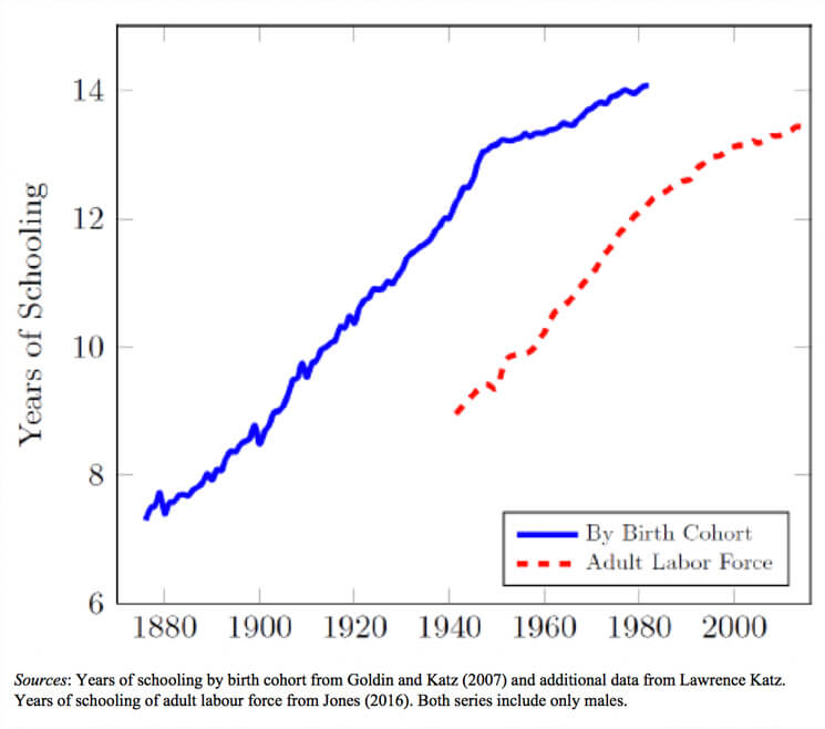
In this setting, capital accumulation raises labour’s income share, holding the supply of skill constant, because the elasticity of substitution is below one. However, as the capital stock grows, the existence of capital-skill complementarity means that workers choose to accumulate more human capital and this effect tends to reduce labour’s income share. For a class of production functions identified in Grossman et al. (2017b), these effects exactly offset one another and the economy has a unique balanced growth path along which labour’s income share is constant. On the balanced growth path, educational attainment rises steadily over time, in keeping with the US experience for much of the 20th century (Figure 1).

Figure 1 US education by birth cohort and among adult labour force

The main outcome of interest is labour’s steady state income share. In the empirically relevant case where the intertemporal elasticity of substitution is less than one, we find that a decline in the rate of either capital-augmenting or labour-augmenting technical progress reduces labour’s income share. Thus, a productivity slowdown induces a decline in the labour share. The mechanism operates through optimal schooling choices. Slower growth reduces the real interest rate, leading individuals to raise their targeted human capital for any given level of the effective capital stock. Since skills are capital-using, this change is equivalent to a reduction in the capital-labour ratio, which redistributes national income toward capital when the elasticity of substitution between capital and labour is less than one.

A productivity slowdown also reduces the rate at which educational attainment increases, but only if it results from a decline in capital-augmenting (not labour-augmenting) technical progress. Figure 1 shows that the increase in schooling in the US slowed for cohorts born after around 1950.

To understand the novelty of these findings, we can compare our results with the canonical neoclassical theory of the functional distribution of income dating back to Hicks (1932) and Robinson (1933). In the canonical approach, where aggregate output is a constant returns to scale function of capital and labour, variation in the labour share results from changes in the capital-labour ratio or in the bias of factor augmenting technologies. If the capital-labour elasticity of substitution is below one, as most empirical evidence suggests (Oberfield and Raval 2014), either an increase in the capital-labour ratio or an improvement in the capital-augmenting technology would raise the labour share.

By contrast, according to our model it is not the levels of technology parameters that determine the labour share, but the rate of technical progress. Moreover, the factor bias of technical progress does not play a critical role in our story. Both a fall in the rate of labour-augmenting technical change and a fall in the rate of capital-augmenting technical change cause a decline in the steady state labour share, because both have qualitatively similar effects on targeted human capital levels.

Quantifying the consequences of a productivity slowdown

How large is the change in labour’s income share resulting from a slowdown in productivity growth? We address this question by calibrating our model to the postwar US economy and simulating a reduction in technical progress that results in a one percentage point per year fall in labour productivity growth. All but one of the parameters can be pinned down using standard data moments such as the capital share, the internal rate of return on schooling, and the growth of labour productivity and years of schooling prior to the shock.

The remaining parameter controls the degree of capital-skill complementarity. To calibrate this parameter, we try two approaches. First, we make ad-hoc assumptions about the bias of technical change. Second, we estimate the parameter structurally using variation in labour shares and average wage growth rates across US states and industries. In all the cases we consider, a one percentage point decline in the labour productivity growth rate reduces labour’s income share by at least 1.5 percentage points. For our preferred specification, the labour share declines by 4.6 percentage points if the slowdown results from lower labour-augmenting technical progress and 5.9 percentage points if slower growth in capital-augmenting technology is responsible.

Conclusions

Our work identifies a new mechanism behind changes in labour’s income share. Moreover, calibrating the model shows that the recent productivity slowdown may be quantitatively important in explaining the redistribution of income from labour to capital.

To conclude, we mention two additional attractive features of our story. First, it does not rely on factors that are specific to the US experience, but instead is consistent with evidence of a global productivity slowdown and a decline in the labour share worldwide. Second, although we focus on recent trends in productivity and the labour share, there is some evidence that similar correlations hold over much longer time periods (Growiec et al. 2016). It is possible that productivity growth and the functional distribution of income have been linked for quite some time.

References

Acemoglu, D and P Restrepo (2016), “The Race between Machine and Man: Implications of Technology for Growth, Factor Shares, and Employment”, NBER Working Paper No. 22252.

Autor, D, D Dorn, L Katz, C Patterson and J Van Reenen (2017), “The Fall of the Labor Share and the Rise of Superstar Firms”, mimeo MIT.

Ben Porath, Y (1967), “The Production of Human Capital and the Life Cycle of Earnings”, Journal of Political Economy 75(4, Pt. I): 352-65.

Elsby, M W L, B Hobijn and A Sahin (2013), “The Decline of the U.S. Labor Share”, Brookings Papers on Economic Activity 47(2): 1-63.

Fernald, J G (2014), “Productivity and Potential Output Before, During, and After the Great Recession”, Federal Reserve Bank of San Francisco Working Paper 2014-15.

Goldin, C and L F Katz (2007), “Long-Run Changes in the Wage Structure: Narrowing, Widening, and Polarization”, Brookings Papers on Economic Activity 38(2): 135-68.

Gordon, R J (2010), “Revisiting U.S. Productivity Growth over the Past Century with a View of the Future”, NBER Working Paper No. 15834.

Gordon, R J (2012), “Is U.S. Growth Over? Faltering Innovation and the Six Headwinds”, NBER Working Paper No. 18315.

Gordon, R J (2016), The Rise and Fall of American Growth: The U.S. Standard of Living Since the Civil War, Princeton: Princeton University Press.

Grossman, G M, E Helpman, E Oberfield and T Sampson (2017a), “The Productivity Slowdown and the Declining Labor Share: A Neoclassical Exploration”, CEPR Discussion Paper 12342.

Grossman, G M, E Helpman, E Oberfield and T Sampson (2017b), “Balanced Growth despite Uzawa”, American Economic Review 107(4): 1293-1312.

Growiec, J, J Muck and P McAdam (2016), “Endogenous Labor Share Cycles: Theory and Evidence”, SGH KAE Working Paper No. 2016/0015.

Hicks, J R (1932), The Theory of Wages, London: Macmillan.

Jones, C I (2016), “The Facts of Economic Growth”, in J B Taylor and H Uhlig (eds), Handbook of Macroeconomics, vol 2A, Amsterdam: Elsevier.

Karabarbounis, L and B Neiman (2014), “The Global Decline of the Labor Share”, Quarterly Journal of Economics 129(1): 61-103.

Kehrig, M and N Vincent (2017), “Growing Productivity without Growing Wages: The Micro-Level Anatomy of the Aggregate Labor Share”, Economic Research Initiatives at Duke Working Paper No. 244.

Oberfield, E and D Raval (2014), “Micro Data and Macro Technology”, NBER Working Paper No. 20452.

Piketty, T (2014), Capital in the Twenty-First Century, Cambridge, MA: Harvard University Press.

Robinson, J (1933), The Economics of Imperfect Competition, London: Macmillan.


Presentation: U.S. Inequality and Recent Tax Changes

Slides from a presentation by Greg Leiserson for a panel “U.S. Inequality and Recent Tax Changes” hosted by the Society of Government Economists on Tuesday, February 20, 2018. In the presentation, Leiserson argues that the recently enacted Tax Cuts and Jobs Act will likely increase disparities in economic well-being, after-tax income, and pre-tax income.

Download the presentation as a pdf.

Income inequality and aggregate demand in the United States

Income inequality has been on the rise for decades in the United States, but a new working paper looks at how that might be affecting macroeconomic activity through the aggregate demand channel.

Income inequality has been rising for decades in the United States. While there are many reasons why this trend may be concerning, one particular worry for economists and policymakers is the effect that it might have on macroeconomic activity through what is sometimes called the aggregate demand channel. The argument is as follows: There is some evidence that the rich save more than the poor. A rise in income inequality implies more income accruing to the rich, a trend that may be depressing overall consumption and in turn lowering aggregate output and employment.

A competing argument, however, focuses on the resulting increase in savings, which could be expected to translate into an increase in investment, raising the capital stock and economic output in the future. In this view, higher income inequality creates some losers, but it leads to an increase in aggregate Gross Domestic Product. Whether the first or the second effect dominates depends on what macroeconomists call general equilibrium considerations, and in particular, on our presumptions about the response of monetary policy to rising income inequality. This column examines those two effects, based on our newly released working paper.

A model of the effect of income inequality on aggregate demand

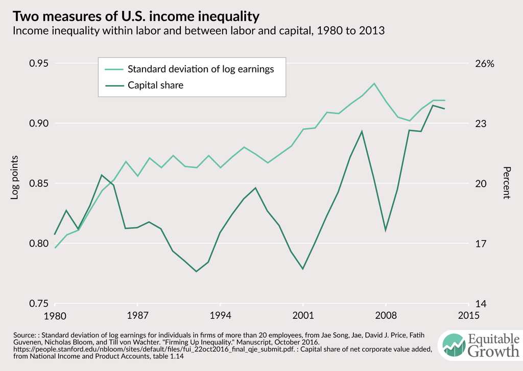
Before turning to that analysis, let us first briefly establish the basis of our inquiry-rising income inequality. Two common measures of inequality in the United States are the standard deviation of log earnings (a measure of inequality within labor income) and the capital share (a measure of inequality between labor and capital). As has been widely documented, both measures have risen since the 1980s.18 (See Figure 1.)

Figure 1

Up until now, most general equilibrium macroeconomic models that were used to evaluate the effects of rising inequality were built under the assumption that the U.S. Federal Reserve would immediately accommodate increases in income inequality by lowering interest rates. Those models accord with the second view-that inequality leads the Fed to lower the cost of capital, encouraging investment, which can lead to an economic boom. In our paper, we show that if we assume that monetary policy has limited willingness or ability to respond to the rise in inequality, then the outcome for GDP looks more concerning.19 Lower consumption lowers employment and individual incomes, feeding back into even lower consumption. Firms disinvest because they anticipate lower employment in the future, and this lowers incomes even further.

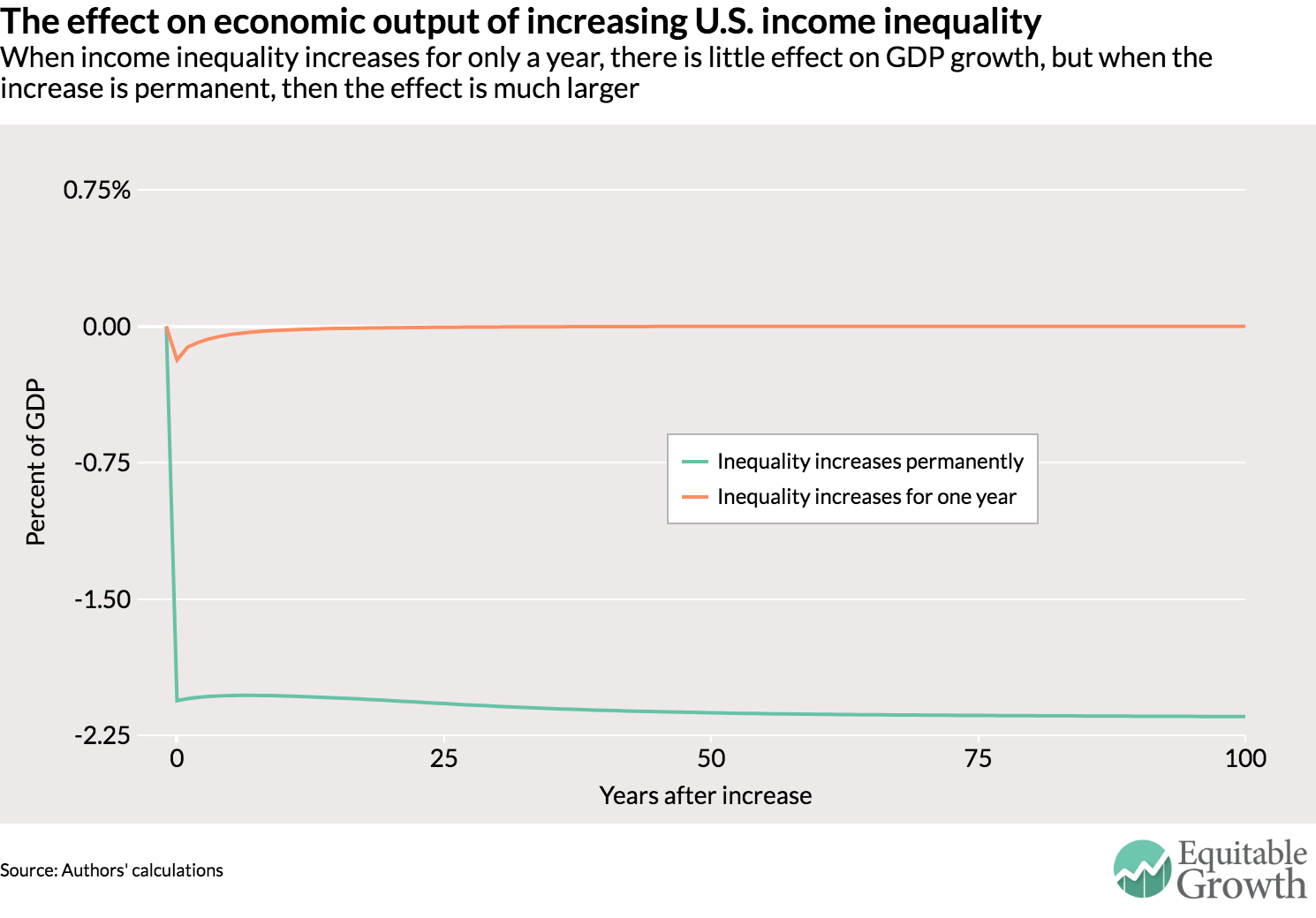
Our new model fits known facts about individuals’ marginal propensities to consume and their saving behavior. We use the model to predict the potential effect of an increase in inequality on economic output, assuming that monetary policy is at the zero lower bound for nominal interest rates, so that it is constrained not to respond to increases in inequality. We show that the key determinant of the effect of inequality on GDP is its effect on asset demand. This is the answer to the question: How much would aggregate wealth increase if we were to artificially hold all other macroeconomic factors such as interest rates and incomes constant? For illustration, we consider two scenarios: one in which inequality rises temporarily-as in the year-to-year fluctuations in the 1990s-and one in which it increases permanently. (See Figure 2.)

Figure 2

In each case, we assume an increase in inequality of four log standard deviation points (the extent to which the light green line in Figure 1 rose since the 2000s). The orange line in Figure 2 shows that if this increase lasts for only a year, then the effect on output is negative but small-less than two-tenths of a percentage point of GDP. The reason is that marginal propensities to consume are negatively correlated with individual incomes, but this correlation is small-a fact that holds not only in our model but also in datasets that have information about individuals’ incomes and marginal propensities to consume. Hence there is a small effect on asset demand, and a small effect on output.

Our more provocative result is the red line in Figure 2-the case of a permanent increase in inequality. There, our model predicts that the level of output could fall permanently by around 2 percentage points as a result. The reason is that inequality causes individuals’ asset demand to rise permanently by a large amount. In our model, this is because inequality leads individuals to face more risk and volatility in their incomes-and that of their offspring-going forward, leading them to increase savings for precautionary and income smoothing purposes.20 In general equilibrium, employment has to fall by a substantial amount to restore equality between the demand and the supply of assets.

Asset demand, asset supply, and equilibrium interest rates

While this is a stark outcome, our new paper suggests ways in which policy can mitigate the effect of income inequality on aggregate demand. The first is fiscal policy, including government spending and budget deficits. In our model, increases in budget deficits help mitigate the fall in economic output because more government debt increases asset supply.

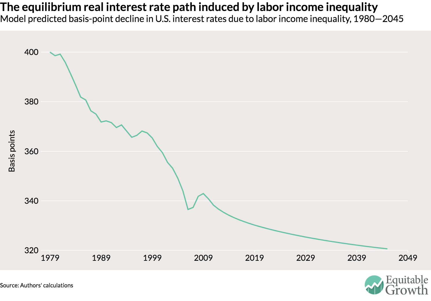
Similarly, monetary policy can respond by lowering interest rates. In fact, the decline in U.S. interest rates that we have observed since the 1980s could have been a response, in part, to rising inequality. Our model predicts what might have been the effect of rising inequality (as in the light green line of Figure 1) on the “equilibrium” or natural interest rate-the interest rate that the Fed needs to set in order to maintain full employment without generating inflation. (See Figure 3.)

Figure 3

Our model suggests a decline of 80 basis points in that equilibrium rate due to rising income inequality, about one-fifth of the 4 percentage point decline documented by Federal Reserve economists Thomas Laubach and John C Williams between 1980 and 2013.21 One implication of our finding is that inequality might have been one of the factors bringing the Fed closer to the zero lower bound of interest rates in the aftermath of the financial crisis beginning in 2008.

Another implication of our demand-supply framework is that of the effect of a rising capital share on equilibrium interest rates and aggregate demand. The dashed red line in Figure 1 shows an increase in that share over the past 30 years. Economists Paul Krugman and Lawrence Summers have argued that this might have contributed to depressing the equilibrium interest rate-or that further increases in market concentration today would be detrimental to aggregate demand.22 In our model, these claims are incorrect. We find that an increase in the capital share always leads to an increase in asset supply because more profits get capitalized into assets that households can trade. This increase in the supply of tradable assets has the exact opposite effect from the increase in asset demand due to higher income inequality: It raises equilibrium interest rates and raises output in liquidity traps.

Policy implications

Our work has a number of important policy implications. First, it suggests that the Federal Reserve and other central banks should keep track of income inequality over time because it influences the decisions that central banks ought to take. Second, our work suggests that not all forms of income inequality have the same effect on equilibrium interest rates: Inequality that raises future risk depresses the natural rate of interest, but technological advances that raise the capital share raise can have the opposite effect. Our model also suggests a more benign view of fiscal deficits than is often assumed in policy discussions because of their beneficial effects on asset supply. A combination of detailed data work narrowing in on the causes of rising income inequality, combined with a model that teases out its aggregate implications, can help the Fed conduct better monetary policy.

Adrien Auclert is an assistant professor of economics at Stanford University and Matthew Rognlie is an assistant professor of economics at Northwestern University. Auclert is a Washington Center for Equitable growth 2015 grantee.

After 25 years, it’s time for paid leave

It has been 25 years since the Family and Medical Leave Act was signed into law by President Bill Clinton, providing unpaid leave for qualified workers. Now it’s time for federal paid family and medical leave legislation.

Twenty-five years ago, barely two weeks after Bill Clinton was sworn in as president, he signed his first piece of legislation: The Family and Medical Leave Act. The law provides most workers with the job-protected right to take unpaid time off from work to care for a new child, a sick family member, or one’s own health. Now, it’s time to update the law to include paid leave.

Since its passage, the Family and Medical Leave Act of 1993 has served as a lifeline for workers, having been used more than 200 million times. But the law alone is not enough to address the needs of families in today’s economy: It only covers 60 percent of workers. Those who are excluded are disproportionately low-income and less educated. And even those who are eligible for unpaid time off do not take it, primarily because of financial reasons. Lack of access to paid leave has long-term economic effects as well, such as lower labor-force participation and reduced lifetime earnings.

That is why Congress needs to pass a comprehensive federal paid family and medical leave policy and the president needs to sign it. Federal policymakers can learn from the experience of the states such as California, New Jersey, and Rhode Island, all of which boast successful state paid leave laws, to craft a policy that is based on evidence garnered in our own backyard.

Last fall, we wrote a paper for The Hamilton Project at The Brookings Institution on the updates to U.S. labor policies that are necessary to address the concerns of 21st century families. In our report, we dug into the research to outline what must be included in a federal paid leave policy that benefits workers and their families while improving broad-based economic growth. Based on the evidence, we proposed that a successful paid leave policy must include the following:

  1. Cover the range of family and medical needs that require time away from work. Much of the discussion today around paid leave centers on parental leave to care for newborn children, but an effective paid leave program must include leave for workers to address their own illness or that of a family member. As the population ages, an increasing number of workers need time off to care for an aging parent or relative. And over half of those who used unpaid leave last year did so to address a personal medical concern.
  2. Be available to all workers, men and women, equally. An effective paid leave program should cover all workers regardless of employer identity or size, or the worker’s full-time or part-time status. It should also use an inclusive definition of family. Furthermore, paid leave should be gender neutral, following the example of the Family Medical Leave Act in providing eligible men and women with the same amount of leave.
  3. Provide adequate length of leave to address care needs. Paid leave should entail at least 12 weeks of leave, allowing families enough time to deal with a serious illness or to care for a new child.
  4. Have a sufficiently high replacement rate to make a difference in people’s lives. Wages should be replaced at a level sufficient to protect families at a time when household expenses rise. We suggest that, at the minimum, a national policy mimics New Jersey’s 66 percent wage replacement with a cap that prevents benefits from being overly generous to high-income families.

Each of these principles is based on evidence from the states, as we detail in our paper. In order to avoid burdening employers, all of the state programs are based on a social insurance system. That means the state governments collect a small payroll tax from employees (and in certain states, employers as well) and then pays out benefits directly to workers. A version of these models could be easily replicated at the federal level.

These policies have been overwhelmingly successful, with these states seeing, for example, increased labor-force participation, hours worked after the birth of a child, and a decline in the use of public assistance to cope with family medical emergencies. To date, there is no evidence that firms experience higher employee turnover or rising wage costs. In fact, a study done by Pew Research Center found that paid leave makes it more likely that workers return to their original employer compared to unpaid leave.

The 25-year-old Family and Medical Leave Act is not enough for workers or the U.S. economy today. A well-designed federal paid leave program based on a social insurance model would benefit U.S. workers and the U.S. economy alike.

In conversation with Richard Reeves

“Equitable Growth in Conversation” is a recurring series where we talk with economists and other social scientists to help us better understand whether and how economic inequality affects economic growth and stability.

In this installment, Equitable Growth’s Senior Director for Family Economic Security and Senior Fellow Elisabeth Jacobs talks with Richard Reeves, senior fellow in Economic Studies and co-director of the Center on Children and Families at The Brookings Institution and most recently the author of Dream Hoarders: How the American Upper Middle Class Is Leaving Everyone Else in the Dust, Why That Is a Problem, and What to Do About It (2017).

[Editor’s note: This conversation took place on October 11, 2017.]

Elisabeth Jacobs: Let’s jump right in, Richard. Who are the dream hoarders?

Richard Reeves: I define them in two ways. One, they are the people at the top of the income distribution who are essentially the winners of the inequality divide in our country, who have risen to the top over the past three or four decades. They are, in my view, the top 20 percent roughly of the income distribution. That means they earn healthy six-figure household incomes, with average incomes of about $200,000 a year.

This is where I see the divide between the bottom 80 percent and the top 20 percent. But then, more specifically, I identify some behaviors among those at the top of the distribution that I think amount to kind of a form of hoarding. In other words, they are kind of overconsuming, or unfairly consuming, some goods or services that actually give them a leg up or give their kids a leg up in a way that perpetuates the inequality that they are currently benefiting from.

Jacobs: What kinds of goods and services?

Reeves: Education and housing are at the top of my list, and the way that they kind of interact with each other. Think about the way the geography of our cities now reflects economic inequality. There has been a slight drop in racial segregation from very high levels but an increase in economic segregation between neighborhoods, between different areas. I think that’s true at the top, as well as the bottom of the income distribution too. So, we are seeing those who are affluent, the top 20 percent and above, separate themselves off into different neighborhoods, which means they can access education resources such as Kindergarten through grade 12 education, and then use local zoning laws to protect the neighborhoods and the land in those neighborhoods from incursions by those who are of more modest economic backgrounds.

That’s all subsidized through the federal mortgage interest deduction. If you want to think about the way in which money buys opportunity and therefore perpetuates inequality, the interaction between the income trends and earning trends, the residential segregation of neighborhoods, the way that education is provided and local zoning laws and regulation of land—they all interact with each other in a way that effectively means the federal government subsidizes me in an expensive neighborhood in an area with great schools. I can then defend against anybody else using unfair exclusionary zoning laws. And my kids therefore get to go to a good public high school and live in a relatively affluent neighborhood.

Jacobs: Why do you think this happened?

Reeves: It’s the combination of millions of small decisions. I think that what happened was that we’ve seen growing labor-market inequality, which combined with inequalities in family formation and family structure and, using a stunningly unromantic phrase, assortative mating, has led to even greater household income inequality. That money, in a society where money matters so much, has been able to be readily transferred into other kinds of advantages, including wealth, including housing, and including access to education.

So, you can see the how. The question then is why, and I think you have to talk about incentives, and the particular incentives of those who are doing well to protect their own position and to protect the position of their children. And I think there is inequality and class perpetuation that really speak to each other.

One of the things I think more strongly now than when I even wrote the book is that actually it’s a long way down from the upper-middle class. It’s a long way down. And the stakes are higher because actually dropping from the 90th to the 50th percentile of income doesn’t look very good down there.

Jacobs: Right.

Reeves: So, being in the middle or lower than that in the United States has dramatic consequences for other things such as access to health care, access to housing, and access to your kids’ education. So it’s both farther to fall and a harder landing, which means the upper 20 percent are highly incentivized to use every means at their disposal to protect their position and the position of their children, and if there are tools available to do that, even if they become exclusionary and unfair, they are highly incentivized at an individual level to use everything, every tool at their disposal. And individually that’s kind of rational, and in some ways sort of justifiable because of this fear of falling, as [author and activist] Barbara Ehrenreich phrases it.

Fear of falling is a really great phrase. The worse inequality gets, the greater the incentives among upper-middle class households to prevent downward mobility and protect their position. The more successfully they do that, the worse inequality gets. I think one other thing that’s important as to why it happens is the more separate these households become, the more their reference point for what counts as rich or affluent changes. It gets distorted because they tend to use local reference points. And it’s much easier to convince yourself you’re not very rich, even if you are in the 95th percentile, if everyone who you know is in the 98th percentile.

This “I’m not rich” problem is getting worse because they are seeing people who are segregated by neighborhood, by institution, by occupation, by marriage, and essentially spending their time more and more with people like themselves or wealthier than themselves. And that actually increases the fear of failure because you don’t see yourself as the winner because you’re always looking up.

This creates real problems as a political way of thinking because it does encourage those who are maybe not quite in the top 1 percent, earning $400,000 or more, to say “I’m not rich. I’m not rich.” Everyone wants to tax the rich, and no one thinks they are rich. And that’s another side effect of economic inequality when it becomes physical, becomes corporal, is incorporated into our neighborhoods and our institutions—so incorporated that it has these huge effects of reference point bias and insulation from what’s really going on. This institutionalization of inequality in the various ways that I’ve talked about speaks to this class divide, and that most troubles me. To me, this speaks to the kind of infantilized debate about inequality, where it’s much easier to stop eating avocado toast than it is to talk about the fundamental problems of the wage distribution.

Jacobs: Part of the problem, too, is the connection between this “I’m not rich” effect and the provision of public services and public goods. Underlying your argument about the separation of classes is that society today doesn’t actually have a unified sense of public goods and have a floor for the quality of public goods in this country.

Reeves: One argument for public goods is it de-risks downward mobility, it lowers the stakes about your own position and the position of your children, and therefore somewhat blunts the incentives to do absolutely everything in your power to protect your position. You can’t get that desperate because the stakes are little bit lower. Therefore, people in the upper-middle class will pull back a bit, be persuaded that actually they need to give up a little bit, and it’s not the end of the world.

Still, for the top 20 percent of households, it does feel like a long way down. When people in the upper-income neighborhood I live in obsess about their kids getting into a good college, and I tend to say, “Relax already,” and they say, “No, it’s different now.” And what they say, it’s because the Chinese are coming, or robots, or whatever—they point to this much more competitive world. But actually I think it is different now, but in a different way. It’s different now because the stakes are higher—that actually failing to get a good start in the labor market will have kind of tougher consequences.

The other thing it speaks to, and you’ve written about this yourself, is the growing importance of human capital of various forms in terms of the labor market. It means you’ve got to do better earlier now. It doesn’t feel as if, well, if you don’t do so well now, then maybe you don’t do so well in college, but you can catch up later. I think the labor market can still do that, but my sense is that it doesn’t do it as effectively as it did before. Unless you hit the labor market with a decent running start in the labor market—and that means increasingly certain qualifications, credentials, human capital, and so on—it’s just tougher to succeed than it was before.

I am making it personal because I think inequality is more personal, that some people are willing to accept as a necessary first step toward saying, “Oh, well, in that case, maybe we do need to do more redistribution. Maybe things aren’t as fair. Maybe actually I could give up a bit more as a necessary first step towards doing that.”

Jacobs: You say in your book that you believe in meritocracy for adults but not for kids. Which is like halfway there, right, but like you still believe in meritocracy for adults?

Reeves: Well, I still basically believe in the market for adults. That invites some criticism from the left, too, because I think the other things being equal, a sort of reasonably freely functioning labor market tends to be relatively meritocratic. I think it has helped to overcome historic prejudices of various kinds, based on gender and race, though there’s still a long way to go. It’s like the alternative to democracy, it’s better than the alternatives.

The idea that social engineers can start deciding that person A is worth more than person B, I think, flies in the face of the evidence of human capital skills. The things that are rewarded in the market tend to be rewarded in the market. It doesn’t mean you can’t then do more to distribute market rewards, but I quite like that. What I don’t like is the fact that the preparation for the market is so uneven. Once the market starts to kick in, it does its thing. So, broadly, the reason why kids of the upper-middle class go on to do so well is not because, by and large, the labor market discriminates wildly in their favor. It does discriminate, but not wildly. It’s because they are chock-full of human capital and skills and credentials, soft skills, hard skills, you name it. They are pretty awesome in the labor market.

The problem is, the idea of meritocracy creeps into childhood. There is selection into our education institutions, even selection into our high schools. That leads to thinking that, well, the brighter kids should get the greater resources, they should get more opportunities. So, the idea of meritocracy kicks in quite early. And if anything, education should be antimeritocratic. If the goal is to equalize the contest, then we need to think about it completely differently and then have the contest.

The other criticism from the left is the top 1 percent. But if one looks at how much real income growth has gone to the 1 percent, and if one uses the share of growth and income accruing to the 1 percent to illustrate the point, then one can produce this amazing chart and say, “This is wrong.” But it’s not just that 1 percent. Some people say, “No, that’s ridiculous, it’s not the top 20 percent, it’s much more like 15 percent, maybe 10 percent.” I say, “Fine, okay, great, big deal.” I’ll take it. I would like to cut the upper-middle income distribution a little bit broader, but I’ll take 10 percent or 15 percent because at least that level is just the 1 percent.

Some people do genuinely still think it is just the top 1 percent who define inequality in the United States. They still have to deal with the fact that individuals and families are moving in and out of the 1 percent quite a lot, but they do still think that that’s the real fracture. There are two kinds of inequality here. There’s a kind of plutocratic inequality and a bourgeois inequality. I think both can be true. You can have the kind of pulling away, not just among the top 1 percent but also the top 0.1 percent. I think within the top 1 percent, there are many who get upset about the 0.1 percent. The 0.1 percent get upset at the 0.01 percent. Every time you add the zero, you just move the class wall a few notches up. The people who fly commercial versus the people who fly first class, and the people who fly on private jets versus the ones who have got their own planes. No matter how high you go, you can always kind of find a class fracture. I don’t think we can just do it on the basis of the top 1 percent.

But in my book, I also examine the danger of the classic “born on third-base thinking you’ve hit a triple” problem. I choose a few examples that get into problems such as legacy preferences in education or the way neighborhoods are zoned or how internships are secured. Because all of that looks like cheating to me. I’m trying to interrupt what I think is a complacent narrative that’s there on the conservative right, which is just, well, they are just amazing people and they are not doing anything wrong.

Jacobs: You talk a lot about legacy admissions, internships, occupational licensing, and exclusionary zoning. Say a little bit more about that and about why you highlighted those.

Reeves: Some of my suggestions about restructuring the financing of higher education, more access to health care, family planning, restructuring K–12, are all highly important and totally unoriginal. There is a vast literature on all of those. We know what need to do. The problem is that we can’t do it. And the reason we can’t do it is because the upper-middle class has convinced themselves that they don’t need to give anything up and that things are hunky-dory, basically. Or they have subcontracted it all out to more distant institutions. They don’t have to do anything personally. I’m trying to interrupt that narrative.

Take the most trivial problem—legacy preferences—and there’s a trivial objection to that, which is made all the time. People say, oh, it won’t make any difference. Great, let’s do it then. So, let’s do that and move on. If it really won’t make any difference, then why are you so worried about it? Why is everyone so troubled about it if it won’t make any difference?

I think the conversation about inequality has to be uncomfortable, and legacy preference is one example of that. It’s outrageous, it’s racist, it’s outdated, it’s a national embarrassment. So you might say, well, if you win that, so what? I would say, if I can’t convince the top of the upper-middle class, these affluent, well-educated liberal Americans that it’s unfair to have a hereditary principle operating in college admissions, then I think the chance of radically transforming the financing of higher education basically is zero.

Jacobs: I’m going to ask one more question. I think the relationship between inequality and mobility is at the heart of what you are getting at. But I think in the American story, race and class are fundamentally interwoven. So, I’m curious how you reflect on that, why you spent so little time on it in the book, whether that was an intentional choice.

Reeves: One of the reasons why that is not a big part of this book is because I am focused on the upper-middle class, the top 20 percent, who remain predominantly white, and are actually whiter than the general population today than they were a few years ago. However, I do think, and I wish now in retrospect that I had said more about the tools that are used to perpetuate class inequality—tools that are racist in origin and remain racist in practice, even if not legally sanctioned.

So, that’s why I’m doing more work now on exclusionary zoning. If you live in a relatively affluent neighborhood, then you don’t have to do that much to change the zoning rules. The status quo favors you anyway. It’s much harder to change things than it is just keep things as they are. And one of the reasons things are the way they are is because of the legacy of racist zoning laws and redlining and so on, which is now being sort of repurposed, I think, to perpetuate class, which again still has racist consequences, even if it is not on its face racist.

I now think there is more to the interaction between the two than I thought. The hardest question, and I think we should stop on the hardest question, is from Hispanic or African American upper-middle class families who ask me, “Do you think that if I am black or Hispanic and I have made it to the upper-middle class, I shouldn’t do everything to help my kids remain there?” That’s one of the hardest questions I’ve had to answer. Because the honest answer is, well, no, I don’t think it is the same. There is a different salience there, and there is a much greater risk of downward mobility for black kids anyway.

Jacobs: We could keep on talking until tomorrow, but you’re right to end on the hardest question.

Reeves: All great questions. Thank you.