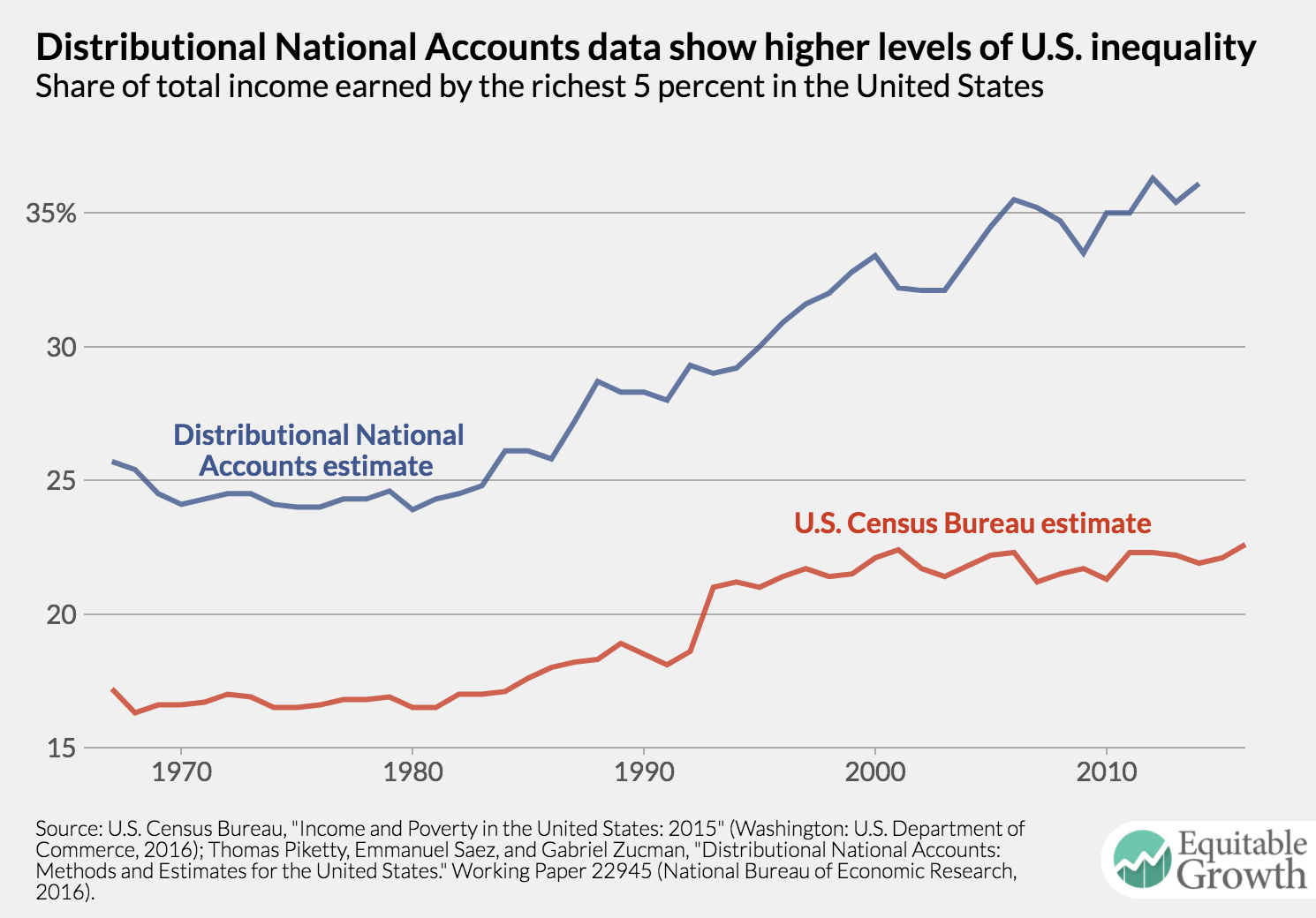
The “Unified Framework for Fixing Our Broken Tax Code” recently released by the Trump administration and congressional Republicans proposes sharp reductions in the corporate tax rate (from 35 percent to 20 percent) and in the tax rate applicable to pass-through income (from 39.6 percent to 25 percent). Proponents of large reductions in the federal statutory tax rates on business income often assert that these cuts will generate large increases in private-sector investment and economic growth. A key premise underlying these arguments is that federal business taxes—the corporate income tax paid by traditional C corporations and the individual income tax paid by owners of pass-through businesses—impose a substantial burden on new investments by businesses.
Yet due to the combination of accelerated depreciation of tangible investments, expensing of intangible investments, largely unrestricted deductibility of interest payments, and the research and development tax credit, federal business taxes impose only a low rate of tax on new investment today. In a recent issue brief, “What is the federal business-level tax on capital in the United States?,” I presented estimates of the effective tax rate on capital income attributable to business-level taxes. The effective marginal tax rate on capital income (the risk-free return attributable to new investment) is 8 percent under current law and would rise only to 13 percent if a temporary provision known as bonus depreciation expires.
Why do new investments face such a low rate of tax attributable to business-level taxes? In short, the answer is that deductions and credits serve to exempt most of the capital income attributable to new investments from taxes. Accelerated depreciation allows businesses to write off the cost of an investment faster than the equipment, structures, inventories, or intangibles in which they invest lose value, effectively understating income. Interest deductions allow firms to subtract interest payments from income, effectively exempting the return on debt-financed investments from business-level taxes. And the research and development tax credit offers a direct reduction in tax for investments in many types of intangibles.
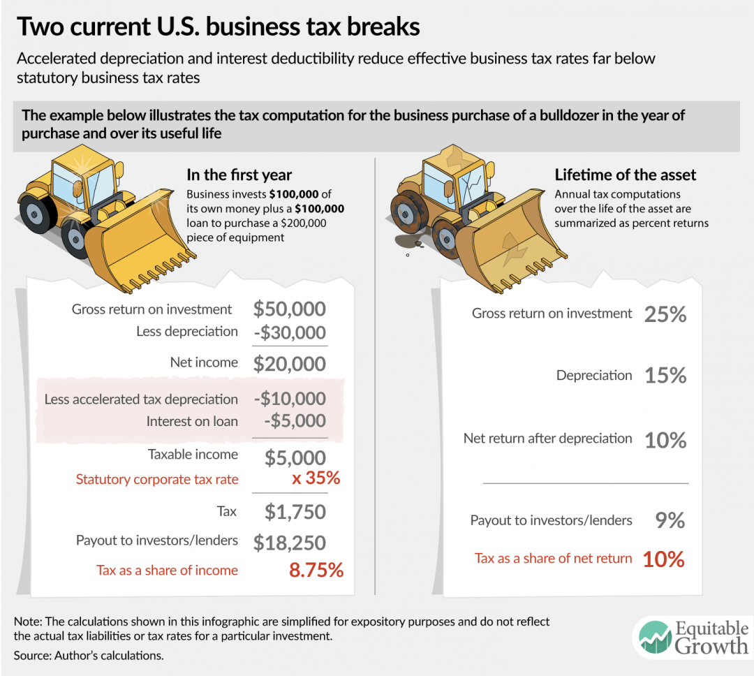
When a firm invests in a tangible asset—for example, when it buys a bulldozer—it is entitled to deduct a portion of the cost of the bulldozer each year to reflect depreciation, or the decline in the value of the bulldozer over time. Depreciation at a rate that corresponds to the true decline in value of the asset over time is referred to as economic depreciation, and depreciation at a faster pace is referred to as accelerated depreciation. Because a dollar today is worth more than a dollar tomorrow, when depreciation deductions are accelerated, it serves to reduce the total tax burden and reduce the tax rate. (See Figure 1.)
Figure 1
On average, depreciation deductions allowed by federal tax law are accelerated relative to economic depreciation. In addition, bonus depreciation—a temporary provision scheduled to expire in 2020—further accelerates depreciation deductions for certain investments. For many types of intangible assets, firms can deduct the full cost of creating them in the year in which the expense is incurred. This extreme case of accelerated depreciation is known as expensing.
In addition to deductions for accelerated depreciation, if a business finances an investment using debt, it can also deduct the interest payments from income. This serves to exempt the income on the debt-financed portion of the investment from business-level taxes. Suppose, for example, a business borrows half the money it needs to buy a bulldozer. Then it will have a stream of interest deductions that offset a portion of the net income generated by the bulldozer equal to the interest payments on that loan. Regardless of whether the interest income is taxed when it is received by the lender, the deduction will serve to ensure that much of the income resulting from this investment does not appear in the business tax base.
Federal tax law also provides a credit for research and development expenses. Similar to other tax credits, the research credit directly reduces the tax rate on the activity for which the credit is granted—in this case, investing in certain intangibles by conducting research.
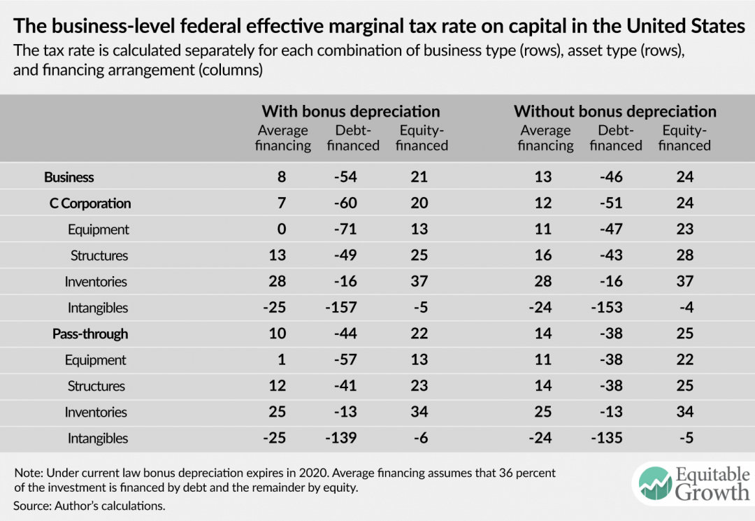
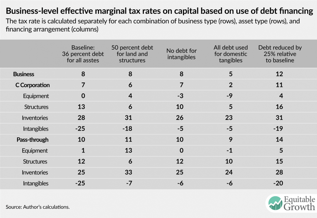
The table below presents estimates of the business-level effective marginal tax rate on capital under current law. The first three columns provide estimates assuming bonus depreciation is in effect and the second three columns provide estimates assuming bonus depreciation has expired. The average business-level effective marginal tax rate is 8 percent under current law today and 13 percent without bonus depreciation, as would be the case for current law in 2020. These rates reflect the average of a strongly negative tax rate for fully debt-financed investment (negative-54 percent) and a positive tax rate for fully equity-financed investment (21 percent). (See Table 1.)
Table 1
A better approach to business tax reform
In light of these findings, the case for reductions in the statutory business tax rate as a means of spurring additional capital investment is weak. A reduction in the business tax rate would come at a very high cost, as it would apply to the entire business tax base, including excess returns and labor income, as well as to returns on investments made in the past. (See this previous column for an extended version of this argument.) The impact on capital investment would be highly attenuated, as debt-financed investments face a negative rate at the business level, and thus a rate cut would increase the tax rate on such investments by reducing the value of the deductions they generate. Moreover, as the channel through which a reduced effective marginal tax rate can increase investment is lowering the cost of capital, deficit-financed tax cuts that increase the cost of capital can be actively counterproductive.
A better approach to reform would focus on reducing the disparities in tax rates across types of produced capital and across financing arrangements. This variation is largely driven by variation in the extent to which tax depreciation is accelerated relative to economic depreciation and variation in the use of debt finance. Well-designed reform should thus pursue a revenue-neutral or revenue-increasing reallocation of the current tax benefits for debt to equity that reduces the disparities in the tax rates on investments in different types of produced capital. Such a reallocation could also lower the tax rate on produced capital and increase the tax rate on land. These reforms would offer a more plausible path to economic growth than reductions in the statutory tax rates on business income.
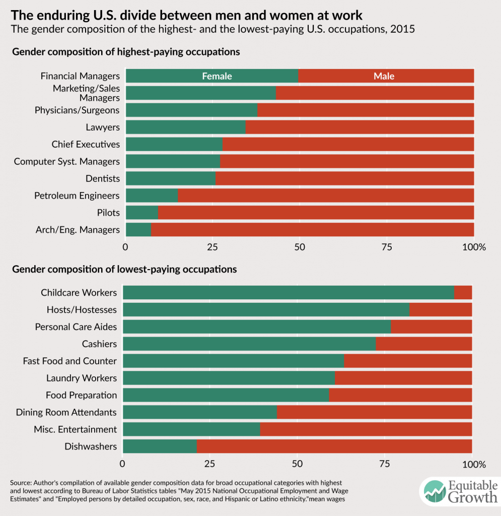
Occupational segregation occurs when one demographic group is overrepresented or underrepresented among different kinds of work or different types of jobs. In 2015, for example, men were 53 percent of the U.S. labor force1, but held less than 30 percent of the jobs in education and more than 98 percent of the jobs in construction.2
The evidence shows that occupational segregation based on gender occurs more because of assumptions about what kinds of work different genders are best suited for than because of an efficient allocation of innate talent. To the extent to which that is true, occupational segregation hurts economic growth because:
It depresses productivity and growth by limiting the economically optimal matching of workers’ skills with jobs.
It depresses the labor force participation rate because workers are less apt to adapt to changes in the economy by taking jobs in growing sectors due to perceptions about which occupations correspond to which gender identifications.
It depresses aggregate demand in the economy by substantially depressing female wages, contributing to the gender wage gap, and therefore reducing families’ incomes.
Key takeaways
Occupations with more men tend to be paid better regardless of skill or education level.3 This is because if work is done predominantly by women, then it is valued less in the labor market. As the rate of women working in a given occupation increases, the pay in that occupation declines—even when controlling for education and skills.4
This trend is also highly racialized: Women of color at all education levels are segregated into jobs with lower wages than their white female peers of similar skill levels.5
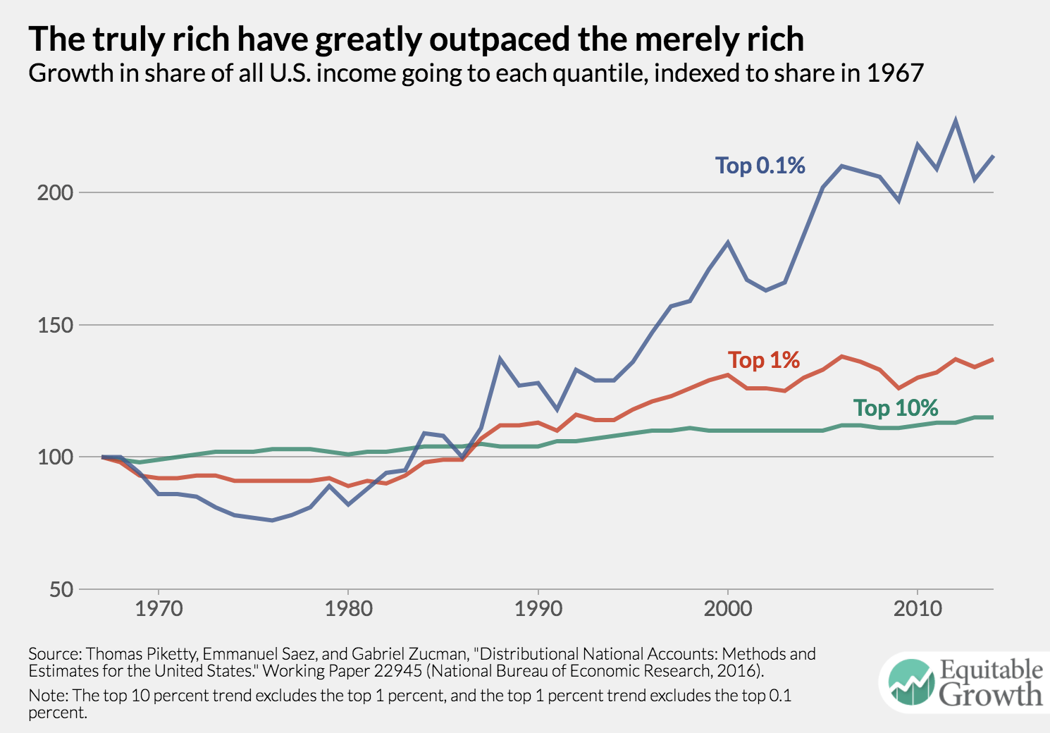
Occupational integration since 1960 was responsible for 60 percent of real wage growth (after accounting for inflation) for black women, 40 percent for white women, and 45 percent for black men.6
Half of the gender wage gap since 1980 can be attributed to women working in different occupations and industries than men, making it the single largest factor. Discrimination accounts for another 38 percent.7
While the prevalence of women in low-paid occupations is due to negative biases about the market value of “women’s work,” the prevalence of men in highly paid occupations is often due to workplace cultures that demand long hours and facetime in the office, which does not accommodate flexibility for caregiving.9 (See Figure 1.)
Figure 1
Many of the occupations that will add the most jobs by 2024, including health care support, administrative assistance, early childhood care and education, and food preparation and services, are composed of more than 60 percent women.10
The shift in the economy from occupations that have traditionally been male-dominated—namely manufacturing—to ones that are female-dominated and low-paid has implications for the structure and strength of U.S. families. As men’s economic position declines relative to women’s, the prevalence of marriage declines and the fraction of children born to poor single-parent households increases.11
To learn more on this subject from the Washington Center for Equitable Growth
“Equitable Growth in Conversation” is a recurring series where we talk with economists and other social scientists to help us better understand whether and how economic inequality affects economic growth and stability.
In this installment, Equitable Growth’s Research Director Elisabeth Jacobs talks to Joan Williams, distinguished professor of law, the University of California, Hastings Foundation chair, and director of the Center for WorkLife Law at the University of California, Hastings College of the Law. They talk about Williams’ book on the white working class.
Elisabeth Jacobs: I’m delighted to be here today with Joan Williams. Joan is one of the first academic grantees co-funded by Equitable Growth for her work with University of Chicago professor Susan Lambert on the business-side impacts of scheduling stability. But we are not here to talk about that today. We are instead here to talk about Joan’s new book, White Working Class: Overcoming Class Cluelessness in America, released by Harvard Business Review Press recently. I’d like to kick off the conversation with the question: Why did you write this book, knowing you are a work-life scholar?
Joan Williams: Well, I basically think of myself as a social inequality scholar. I’m chiefly known for my work on gender, but I have also done a lot of work on how the experience of gender bias differs by race. And I have studied social class for 40 years. I married into a white working-class family in 1978, so I have been thinking a lot about how to bridge what I call the class culture gap between the professional, managerial elite and the white working class.
Jacobs: You’ve chosen to write this book about the white working class for all kinds of reasons. But how many of the things in your book do you think are about the white working class per se, and how many of them are actually more broadly applicable to a very diverse working class? African American families have struggled with many of the challenges.
Williams: There are so many overlaps between the white working class and the working class of color. The need and intense desire for stable jobs that will yield a modest middle-class standard of living is not a white working-class thing, it’s something that appeals to nonelites of all races. That’s why it should be such a central concern for both political parties.
The culture wars reflect that there exist a very different set of cultural dispositions among elites and nonelites. Elites value artisanal coffee. Gender roles. Spiritualities. You name it. Among nonelites, the search is less for novelty than for stability, so nonelites of all races put a high value on institutions that anchor stability, including the military, religion, and family values.
All that produces cultural conflict, but it’s not between the elite and the white working class. It’s between the elite and everybody who’s not elite—poor and middle class of all races. The elites often talk disrespectfully of the cultural truths of nonelites—that’s one of things that’s coming back to bite society.
Jacobs: You talk a lot about how, for white working-class people, their social networks, their kin structures, their lives are very much place-based in a way that means that the expectation that people just move to better jobs and the sort of head-scratching by economists about “why don’t people just move to where the jobs are” doesn’t make a lot of sense, if you think about it in the context of people’s social-cultural lives.
From an economic perspective, it doesn’t make much sense, and I think your work is kind of answering why this decline in labor mobility and decline in economic dynamism in the United States might be an economic puzzle, but in some ways, the sociology of it answers the questions.
Williams: Elites have what are called entrepreneurial networks—wide circles of acquaintances that are often national, or even global. And that’s how 70 percent to 90 percent of professionals get jobs. Working-class and poor people typically have place-based clique networks of family, neighbors, and friends they’ve known forever. Nonelites rely on these clique networks to protect them from their disadvantaged market position, by providing childcare, elder care, and help with things such as home repairs.
So, for moving to make sense, nonelites need not only to find a better job; they need to find one that’s so much better that they come out ahead, despite the fact they now have to pay for childcare and elder care because no family is close enough to help out. Another reason nonelites are reluctant to move is that their social honor is not portable. I was just living in the Netherlands; all I had to do is say I am a law professor teaching at one of the leading Dutch universities for people to want to get to know me. I tell the story in my book about going back to a high school reunion in a working-class town, and having someone ask a former classmate what he did for a living. The classmate got very red and snapped, “I sell toilets!” If your job is inglorious, you want to stick around people who know you, and know that you’re a person to be reckoned with—not just a guy who sells toilets.
Another important point: If you’re working class, the people in the communities you’re moving to have the same kind of dense place-based networks you have—and they’re going to make sure that good jobs go to people in their networks, not to you. This is just the kind of erasure of the realities of people’s lives on the ground that, if I can say this respectfully, economists are so good at.
Jacobs: So, what do you do about that? You often speak about the need for upskilling through non-college-based credentialing and vocational education. But what do you do if people are in places where there aren’t jobs? You can upskill all you want, but if the jobs aren’t there, there’s still the question of how do you make the jobs show up?
Williams: We need a new education-to-employment system that builds alliances between community colleges, local universities, and unions that set up alliances with local businesses, some of them existing, some of them attracting new businesses, so that the businesses can depend on a steady supply of certificate-trained workers with the specific job skills that are needed for their jobs. The goal should be certificate programs that are far shorter than a four-year degree, offered on family-friendly schedules because workers will need to retrain not once, but often several times, for new jobs, as old jobs morph or disappear. This idea and many others come from a very important book out of a Markle Foundation working group, and the book is called America’s Moment, and the initiative is called Rework America. Part of the reason American politics has turned so bitter is that America did globalization wrong, resulting in the loss of many middle-class jobs. We need to do automation right.
Jacobs: That seems like a good note to wrap on. Thank you so much.
Distribution tables—estimates of who wins and who loses from changes in tax law—are central to any debate about tax reform. Such analyses frequently show the plans put forward by Republican politicians to be severely regressive, delivering large income gains for high-income families and little for the overwhelming majority of families. The blueprint for tax reform released by House Republicans in 2016, for example, would increase after-tax incomes for the top 1 percent of families by 13 percent in the first year after enactment but would increase incomes for the bottom 95 percent of families by less than half of 1 percent.
In response, proponents of regressive tax plans often assert—either implicitly or explicitly—that distribution analysis is flawed and fails to account for the benefits of the additional economic growth that the plans would purportedly generate. This view is mistaken. A traditional distribution analysis provides an approximation of the change in economic well-being resulting from a change in tax law. Distribution analysis is thus useful precisely to determine whether tax reform delivers gains for people across the income distribution or only for those at the top.
In the special case of revenue-neutral reform—an ostensible target for current reform efforts in Congress—distribution tables capture the primary gains from increases in economic efficiency in their estimates of changes in after-tax income. In the case of revenue-losing reform, distribution tables overstate the gains from reform, as apparent increases in after-tax incomes will ultimately need to be clawed back through offsetting tax increases or spending cuts. Only in the case of revenue-raising reform will distribution tables understate the gains. Thus, in the most likely cases for tax legislation this fall, distribution tables will either reflect or overstate the gains from any increases in economic efficiency, to the extent they exist at all.
Simply stated, invocations of growth cannot be used to wave away regressive distribution results. Reforms such as the 2016 House Republican blueprint would boost incomes for high-income families at the expense of working- and middle-class families. As Republicans in Congress and the Trump administration continue to develop a proposal for tax reform, it is worth revisiting in this column—and an accompanying issue brief—why traditional distribution tables are precisely the analytical tool they will need to determine if their tax reform plan does, in fact, deliver equitable growth.
Distribution analysis estimates the change in tax burden resulting from a change in tax law assuming no change in behavior. These estimates of the change in the tax burden can then be used to compute a range of summary statistics, including the average tax change, the percentage change in income, or the percent of families getting a tax cut or tax increase for various subgroups of the population.
Critics of distribution analysis often point to the assumption that behavior does not change when tax reform is enacted as a flaw in the analysis. Yet the assumption that behavior is unchanged provides a better approximation of the change in economic well-being resulting from a proposal than allowing behavior to change because the behavioral responses have little direct value to the people changing their behavior.
Why are the behavioral changes of little direct value to families? Because families generally do the best they can in the economic circumstances in which they find themselves; modest changes in behavior due to tax reform do not change their own well-being much at all. If the behavioral changes were to matter a great deal, then it would imply that families were knowingly making choices against their own interest—such as turning down good job offers—before tax reform.
While distribution analysis is appropriately conducted under an assumption of fixed behavior, that does not mean there are no potential economic benefits from behavioral changes that result from tax reform. Gains are possible, but they primarily manifest through their impact on the government budget. For instance, if people change their consumption patterns in response to a new limitation on an unjustified tax expenditure that finances a rate reduction, then those changes will generally improve the government’s fiscal position. This improvement in the government’s fiscal position will make it possible for legislators to provide what appears to be a net tax cut under the assumption of unchanged behavior at no cost to the government. In other words, if a revenue-neutral tax reform plan generates increases in economic efficiency, then the distribution analysis will show a net tax cut even if the cost of the tax reform to the government is zero.
It is precisely legislators’ choices about how to design a tax plan that will determine how that free-to-the-government tax cut is allocated across the income distribution. Indeed, it should not be surprising that the impact of changes in public policy are determined by legislators’ choices about how to change public policy. Recognizing that the potential gains in economic well-being for U.S. families derive from how legislators choose to distribute tax cuts made possible by improvements in the government’s fiscal position appropriately places the focus on the choices legislators make.
Focusing on growth in economic output rather than changes in well-being as measured by distribution analysis not only ignores the potential for tax reform to have different impacts across the income distribution, but also overstates the economic gains from reform by counting increased output as a benefit without accounting for the costs of generating that output. Indeed, the greater risk in the coming months is not that distribution analysis will understate the gains from tax reform, but rather that distribution analysis will overstate the gains and understate the regressivity due to its treatment of increased borrowing should policymakers turn from revenue-neutral tax reform to tax cuts.
Distribution tables—estimates of who wins and who loses from changes in tax law—are central to any debate about tax reform. Such analyses frequently show the plans put forward by Republican politicians to be severely regressive, delivering large income gains for high-income families and little for the overwhelming majority of families. The blueprint for tax reform released by House Republicans in 2016, for example, would increase after-tax incomes for the top 1 percent of families by 13 percent in the first year after enactment but would increase incomes for the bottom 95 percent of families by less than half of 1 percent.12
In response, proponents of regressive tax plans often assert—either implicitly or explicitly—that distribution analysis is flawed and fails to account for the benefits of the additional economic growth that the plans would purportedly generate.13 This view is mistaken. A traditional distribution analysis provides an approximation of the change in economic well-being resulting from a change in tax law. Distributional analysis is thus useful precisely to determine whether tax reform delivers gains for people across the income distribution or only for those at the top.
In the special case of revenue-neutral tax reform—an ostensible target for current reform efforts—distribution tables capture the primary gains from increases in economic efficiency in their estimates of changes in after-tax income. In the case of revenue-losing reform, distribution tables overstate the gains from reform because apparent increases in after-tax incomes will ultimately need to be clawed back through offsetting tax increases or spending cuts. Only in the case of revenue-raising reform will distribution tables understate the gains. Thus, in the most likely cases for tax legislation this fall, distribution tables will either reflect or overstate the gains from any increases in economic efficiency, to the extent they exist at all.
Simply stated, invocations of economic growth cannot be used to wave away regressive distribution results. Reforms such as the 2016 House Republican blueprint would boost incomes for high-income families at the expense of working- and middle-class families.
Focusing on changes in economic output rather than on the distribution of economic gains and losses not only ignores the potential for tax reform to have different impacts for people up and down the income ladder, but also overstates the economic gains from reform by counting increased output as a benefit without accounting for the costs of generating that output. Indeed, the greater risk in the coming months is not that distribution tables will understate the gains from tax reform, but rather that distribution tables will overstate the gains of reform and understate its regressivity if policymakers turn to tax cuts rather than tax reform and include a slate of temporary policies such as a one-time tax on overseas profits.
As Republicans in Congress and the Trump administration continue to develop a proposal for tax reform, it is worth revisiting why traditional distribution tables are precisely the analytical tool they will need to determine if their tax reform plan does, in fact, deliver equitable growth. This brief first explains why static distribution tables are informative about the improvements in economic well-being resulting from revenue-neutral tax reform. It then identifies three reasons that distribution tables may overstate the gains from reforms. Specifically:
Distribution tables typically do not impose budget balance on the policy changes they assess, which means that in the case of deficit-financed tax cuts, a distribution table will show gains attributable to increased borrowing even though that borrowing must ultimately be financed with spending cuts or tax increases that would make families worse off.
Timing gimmicks can affect distribution tables just as they can affect revenue estimates. A one-time tax on the repatriation of overseas corporate profits, for example, could reduce the apparent regressivity of a tax cut if distribution tables are estimated only (or primarily) for years in which the temporary policies are in effect.
If tax reform increases the federal budget deficit, then traditional approaches to measuring the incidence of certain reforms may be invalid.
Despite these limitations, distributional analysis will be critical in understanding the potential gains of any tax reform plan put forward by congressional Republicans and the Trump administration in the coming months. An understanding of what distribution analysis does and does not measure will be essential for policymakers and the public.
Distribution tables reflect the economic gains from revenue-neutral tax reform
To estimate the approximate change in economic well-being from a change in tax law, a static distribution table computes the change in tax burden assuming no change in behavior. The distribution tables produced by the Tax Policy Center and the U.S. Treasury’s Office of Tax Analysis are of this type.14 Assuming unchanged behavior provides a better approximation to the change in economic well-being resulting from a proposal than allowing behavior to change because the behavioral responses have little direct value to the people changing their behavior.15
This perhaps counterintuitive conclusion arises from the analytical assumption that people are always doing the best that they can in the economic circumstances they face. From this assumption, it follows that people equate the gains from small changes in behavior to the costs of those changes in making choices about work, consumption, and savings. If they did not do so, then there would be a small change in behavior that made them better off.
As a concrete example, consider workers earning $20 an hour, working 40 hours per week, and facing a 25 percent tax rate. Under current law, the workers’ after-tax wage is $15 per hour. The maintained assumption is that the workers could choose to increase or decrease their hours slightly at this wage rate if they wished to do so. As they choose not to, then the value to the workers of that additional $15 is roughly equal to the costs of working more such as increased commuting costs, childcare, or less time for household chores. If the cost of working that additional hour exceeded $15, then reducing hours would make them better off. If the cost were less than $15, then increasing hours would make them better off.
If the tax rate for these workers is reduced to 20 percent and the workers decide to pick up an additional two hours per week, then the net value of those hours to them is not the full $32 in additional take-home pay from working more, but rather only about $1. The reason: At the new, higher number of hours worked, the cost of working longer is roughly $16, again equal to the take-home pay. The total cost of work for those two hours would be roughly $31, or about $15 for the first hour and $16 for the second, leaving our hypothetical workers with only an extra dollar to show for the effort.
Notably, the change in well-being resulting from the behavioral response of these workers to a 5 percentage point reduction in the tax rate is far smaller than both the direct impact of the tax cut ($40 in reduced income taxes) and the impact of the change in behavior on government revenues ($8 in new revenue resulting from the increased working hours: 20 percent of the $40 in additional gross pay).
The economic logic of this simplified example generalizes to other choices about work, consumption, and savings. For a small change in tax rates, changes in behavior provide essentially no direct benefits. For a larger tax change, the value of the change in behavior would tend to be small relative to the other effects of the proposal. Note, however, that the conclusion that a family is approximately indifferent to changes in behavior applies only to changes in behavior under its control and only for those decisions where the family is unconstrained in its choices. In more complex models, the relevant assumptions could fail in other ways such as through informational imperfections.
The above analysis treats the conclusion that changes in behavior provide little direct benefit as a justification for static distribution tables, but an alternative and likely preferable mode of analysis would be to determine the types of behavior that should be held fixed in a distribution table as precisely those for which small changes leave families indifferent. Changes in behavior that do not satisfy this property should be included, though the details of doing so can be complex. In fact, implicitly, static distribution tables typically allow at least one form of behavioral response: a switch from claiming the standard deduction to itemizing (or the reverse). One justification for including such changes is that they are essentially costless and thus there is no offsetting cost to the gains delivered by making such a change.
The assumption of no (or extremely limited) changes in behavior used in a static distribution table differs from the behavioral assumptions used in both a conventional revenue estimate and a dynamic revenue estimate. A conventional revenue estimate allows for microeconomic behavioral responses—responses that do not change macroeconomic aggregates such as labor hours or the capital stock. For instance, a decrease in the use of an itemized deduction in response to a limitation on that deduction would be a microeconomic behavioral response. A dynamic revenue estimate allows for microeconomic behavioral responses and changes in macroeconomic aggregates. Because the behavioral assumptions underlying a static distribution table and a revenue estimate are not the same, the aggregate tax change shown in a distribution table will not necessarily match the revenue estimate under either conventional scoring or dynamic scoring.
This gap between the revenue estimate for a proposal and the implied aggregate change in tax liability per the distribution table captures the primary economic gains from a proposal. If tax reform delivers positive revenue feedback—whether through microeconomic behavioral responses included in a conventional score or macroeconomic behavioral responses included in a dynamic score—then the revenue cost of the proposal will be smaller than the tax cut implicit in the distribution tables. An efficiency-enhancing tax reform that is revenue neutral including dynamic feedback would thus show a tax cut in the distribution table at no revenue cost to the government. That free-to-the-government tax cut reflects the primary economic benefits of the reform.
Consider a second example. Suppose a person making $50,000 and facing a tax rate of 25 percent can deduct from income certain expenses equal to $10,000. The government then replaces the deduction with a 20 percent tax credit and provides a $900 tax credit instead. The individual responds by reducing spending on the deductible expenses to $8,000. The government collects the same amount of revenue under this reform as it would under current law. In other words, the revenue estimate is zero.
Moreover, because the amount of the deductible expense was chosen freely prior to the reform, the person was roughly indifferent between an additional dollar of the deductible expense and nondeductible expenses. This will remain approximately the case after the reform, and thus the person realizes only a very modest gain from the behavioral change. Importantly, however, the new tax credit is worth $900 and the limitation on the deduction costs only $500 (before the reduction in such spending), which means the distribution table would show a net tax cut of $400 that was provided at no net cost to the government.
In other words, if policymakers can deliver tax reform with real economic benefits that is revenue neutral on a dynamic basis, then an appropriately constructed distribution table for that tax reform would show a net tax cut. And if the tax reform delivers equitable growth in living standards, then the table will show robust increases in well-being for working- and middle-class families, as well as high-income families.
The validity of the static distribution as a measure of the change in economic well-being also highlights the role of government policy in determining the way the economic gains from tax reform are translated into increases in well-being for families up and down the wealth and income ladders. As the behavioral changes resulting from tax reform are of relatively little direct value to families and the broader efficiency gains generally arise from the impact of reform on the government budget, it is government policy that determines how those gains are allocated. Notably, since the behavioral changes are of relatively little direct value to families, if the static tax cuts are concentrated among high-income families, then growth will not change that fact.
Of course, static distribution tables remain an approximation to the change in economic well-being, and there is plenty to debate about their construction. The quality of the approximation declines as the rate change gets larger, though for a revenue-neutral reform, the overall rate change should be small. A higher-quality approximation would show slightly higher benefits of efficiency-enhancing reform.16 Many of the assumptions underlying a distribution table and the associated revenue estimates are uncertain such as the responsiveness of labor supply to tax changes and the allocation of the incidence of the corporate income tax to labor and capital. Changes in wage rates and investment returns resulting from behavioral responses can affect the results. Distribution tables do not capture the benefits or costs of simplification proposals, though these are typically modest. Interactions between federal and state revenue streams often receive insufficient attention in federal policymaking.
There is much to debate about the details of distribution tables, but their importance in assessing changes in economic well-being is clear. Static distribution tables provide a reasonable approximation to the change in economic well-being across the income distribution, and economic growth does not. If revenue-neutral tax reform delivers equitable growth, then a static distribution table will show it.
Distribution tables are more likely to overstate the gains of reform
The greater analytic risk in the coming months is not that distribution tables will understate the gains from reform, but rather that they will overstate the gains from reform and understate its regressivity.
First, as noted above, distribution tables typically do not impose budget balance on the policy changes they assess. In the case of deficit-financed tax cuts, a distribution table will thus show gains attributable to increased borrowing even though that borrowing must ultimately be financed with spending cuts or tax increases. Incorporating those offsetting fiscal policies into the analysis would reduce the apparent gains in the distribution table. In fact, the primary scenario in which static distribution tables understate the gains from tax reform is one in which Congress enacts tax reform that is revenue neutral on a conventional basis and uses the economic gains to reduce the deficit and debt. In this case, the distribution table would show a near-zero change in well-being even though gains have been realized.
Second, timing gimmicks can affect distribution tables just as they can affect revenue estimates. A time-limited policy such as a one-time tax on the repatriation of overseas corporate profits could reduce the apparent regressivity of a tax cut if distribution tables are estimated only or primarily for years in which the temporary policies are in effect. More broadly, practical considerations make the construction of distribution tables on a present-value basis difficult, but there would be substantial analytic value to such an exercise. In the absence of a present-value analysis, caution is required in interpreting distribution tables for policies that differ substantially across years or for which a substantial adjustment period is likely.
Third, if tax reform increases the federal budget deficit, then traditional approaches to measuring tax incidence may be invalid. Distribution tables, for example, typically assign a portion of the incidence of a corporate tax cut to labor and a portion to capital. Most analysts assume a partial pass-through to labor based on anticipated changes in the capital stock. But the capital stock will change only over time, and whether it will grow—and whether that growth will be sustained—depends on whether increased federal budget deficits drive up interest rates and discourage private-sector activity. Thus, deficit financing not only can reverse short-run gains from a proposal and ultimately harm growth, but can also result in misleading distribution estimates that assume labor benefits from capital deepening even as the proposal reduces the capital stock.
As Congress turns its attention to tax reform, dramatic reductions in the top statutory tax rates on business income are sure to be among the most important and most contentious elements of the debate. Under current law, the top statutory tax rate for traditional C corporations is 35 percent, and the top statutory tax rate for pass-through businesses is 39.6 percent. The Trump administration has proposed a top rate of 15 percent rate for both C corporations and pass-through businesses, and Republicans in the U.S. House of Representatives have proposed a top rate of 20 percent for C corporations and 25 percent for pass-through businesses.17
Proponents of these sharp rate cuts often justify them by arguing that they will increase investment and thus economic growth. In a wide class of economic models, however, the statutory tax rate on business income has no direct relationship to investment or growth. It is instead the effective marginal tax rate on capital that most closely relates to the level of investment. The effective marginal tax rate relevant for investment decisions includes the impact of business-level taxes, investor-level taxes, and lender-level taxes. Statutory tax rates on business income only influence the portion of the effective marginal tax rate attributable to business-level taxes.
The business-level federal effective marginal tax rate on capital depends on many complex provisions of the tax code in addition to the statutory tax rate, including the rules governing the depreciation of business assets, the availability of deductions for interest payments, and tax credits for research and development. The tax rate on an investment varies depending on whether the firm making that investment is a C corporation or a pass-through business, on the amount of the investment financed using debt or equity, and on the assets that make up the investment. Businesses that rely on intellectual property for most of their income, for example, face very different tax rates than those that derive most of their income from rents on real estate—reflecting differences in their ability to benefit from different business tax breaks and in their ability to obtain debt financing for their investments.
This issue brief answers a key question facing policymakers as they debate changes in business taxation: What is the business-level federal effective marginal tax rate on capital today? The analysis in this brief finds that the average effective marginal tax rate is only 8 percent under current law, far less than the statutory tax rates on business income.18 The rate would rise to only 13 percent if a tax break known as bonus depreciation expires in 2020, as scheduled under current law.
Even though little tax is imposed on capital income at the business level, taxes on business income still raise substantial revenues because a large portion of the business-income tax base consists of excess returns (returns above the risk-free rate such as those due to monopoly pricing power), income attributable to labor that was not paid out as wages, and luck. These sources of business income are not included in the definition of capital income used in this brief, consistent with the definition of the effective marginal tax rate on capital, discussed in greater detail below.
While the average business-level effective marginal tax rate is low, rates vary widely for investments in different assets and for investments financed with different proportions of debt and equity. The tax rate on investments in inventories, for example, is 28 percent—relatively close to the statutory rates on business income—while the tax rate on investments in intellectual property is negative-25 percent, meaning an investment would yield excess deductions or credits that could be used to offset taxes owed on other income subject to certain limitations. Similarly, the tax rate on equity-financed investment is 21 percent, while the tax rate on debt-financed investment is negative-54 percent.
Given the low average effective marginal tax rate, it makes little sense to prioritize cutting statutory tax rates. Cutting the statutory tax rates on business income would do relatively little to encourage additional investment and thus have relatively little effect on growth, even before considering the effects of increased deficits resulting from the rate cuts or additional policies to offset that cost. Moreover, the tax cut resulting from a reduction in the statutory tax rates on business income would be severely regressive.
Instead, the combination of a low average effective marginal tax rate and substantial variation in rates for different investments means that there is an opportunity to pursue a superior approach to reform that would focus on reducing the disparity in tax rates between investments and thus generate a more efficient mix of investment projects.
More concretely, rather than cutting statutory tax rates, Congress should pursue a revenue-neutral or revenue-increasing reallocation of the current tax benefits for debt to equity that reduces the disparities in the tax rates on investments in different types of produced capital: equipment, structures, inventories, and intangibles. Such a reallocation could also lower the tax rate on produced capital and increase the tax rate on land. These reforms would offer a more plausible path to economic growth than reductions in the statutory tax rates on business income.
Federal taxation of business income
Income derived from business activity is subject to a complicated set of interconnected taxes. U.S. businesses can be structured as either traditional C corporations or as pass-through businesses. Traditional C corporations pay corporate income tax on their profits. Pass-through businesses—including S corporations, partnerships, and sole proprietorships—are not subject to the corporate income tax. Instead, owners of pass-through businesses pay tax on their share of the businesses’ profits as part of the computation of their individual income-tax liability. The choice between corporate and pass-through form is largely at the discretion of the owners. While the two forms impose different legal requirements and result in different legal and tax treatments, both forms are common and appear in a wide range of industries.
Dividends paid by C corporations are subject to tax at the individual level, but dividends or other distributions from pass-through entities are generally not subject to tax at the individual level. Investors in any type of business who sell an ownership stake that has increased in value realize a capital gain and pay tax on the resulting income. Lenders to any type of business pay tax on interest payments received from the business.
The corporate income tax and the individual income tax rely on similar measures of business profits for determining the tax on corporate income and pass-through income, respectively. Profits are defined as receipts less the cost of goods sold, employee compensation, operating expenses such as accounting and legal services, depreciation, and interest payments.19 The corporate income tax has graduated rates, but the top rate of 35 percent applies to the overwhelming majority of corporate income. Income derived from pass-through businesses is subject to tax according to the progressive rate schedule for the individual income tax.
In addition to the statutory tax rate on business income, the key determinants of the effective marginal tax rate on capital are the rules governing cost recovery, interest deductibility, and the research credit. Each of these components is examined in turn below.
Cost recovery
Cost recovery refers to the quantity and timing of depreciation deductions allowed for capital expenditures such as the purchase of new equipment or buildings. If a business can immediately deduct the cost of a capital expenditure, then the investment is said to be expensed. If a business can deduct only a portion of the cost each year over a multiyear period, then the investment is said to be depreciated. Depreciation at a rate that corresponds to the decline in value of the asset over time is referred to as economic depreciation, and depreciation at a faster pace is referred to as accelerated depreciation. Economic depreciation is required for the proper measurement of income. Under a system of economic depreciation, depreciation deductions correspond to the decline in value of the assets owned by the business, and thus sales less operating expenses and depreciation yields an accurate measure of the income generated by the business. A tax system that follows economic depreciation and has no other special deductions or credits would impose a business-level tax on equity-financed investment equal to the statutory tax rate.
Under current tax law, most investment in equipment and structures is eligible for accelerated depreciation, and most investment in intangible assets such as research and development is expensed. Both accelerated depreciation and expensing reduce the tax rate applied to capital income because deductions are allowed before the corresponding loss due to a decline in the value of the underlying asset. Because a dollar today is worth more than a dollar tomorrow, the value of the reduction in tax today exceeds the value of the future increase in tax, even though the nominal amounts are the same. In contrast to the treatment of equipment and structures, no depreciation deductions are allowed for land or inventories.
To illustrate how these calculations work, consider a simplified example involving the business purchase of a truck. Suppose the truck is expected to last for 8 years. A business that purchased the truck for $20,000 might depreciate it for accounting purposes over that 8-year period, deducting $2,500 from income each year. In contrast, the tax code allows businesses to write off trucks over 5 years. The business could then deduct $4,000 each year for 5 years and recover the value of the investment in the truck over a shorter period.20 Because the deductions are accelerated relative to the decline in value of the asset, they serve to reduce the tax rate on the income generated by the asset.
Depreciation of most equipment and software investment is further accelerated as a result of a temporary provision of law known as bonus depreciation. Bonus depreciation, which has been in effect since 2008, allows businesses to expense a percentage of equipment and software investment and then depreciate the remainder under the usual schedule. Under current law, bonus depreciation is available at a 50 percent rate in 2017, 40 percent rate in 2018, and 30 percent rate in 2019. Bonus depreciation expires in 2020.
Interest deductibility
The measure of business profits subject to tax under either the corporate income tax or the individual income tax consists of receipts less the cost of goods sold, operating expenses, depreciation deductions, and interest payments. As discussed above, economic depreciation is necessary for the proper measurement of capital income, and accelerated depreciation serves as an investment incentive. In contrast, interest deductions serve to assign the legal responsibility for paying tax on capital income to the lenders financing the activity instead of the business owners. As such, they have no direct relationship to the measurement of capital income generated by the underlying business activity. Because the deductibility of interest allows businesses to provide a return to lenders without paying any tax on the income that generated that return at the business level, it reduces the taxation of capital at the business level.
Consider a hypothetical tax system with economic depreciation and full interest deductibility. A firm finances an investment project solely with debt and realizes a return equal to the interest rate paid on the loan. The deductible interest payments would exactly offset the income from the investment such that the business’s income for tax purposes would be zero in every year and thus there would be no business-level tax on that investment.21
If all businesses and lenders were taxable at the same rate, repealing interest deductibility for businesses and exempting interest income from tax would reassign the legal responsibility for paying tax to business owners rather than lenders without changing the overall level of tax, including both the business- and lender-level taxes. (In practice, interest deductions reported by businesses exceed taxable interest income reported by lenders, suggesting that substantial interest income is avoiding tax at both levels.) For the purposes of evaluating proposals for reduced statutory tax rates on business income, however, the distinction between taxation at the business level and the lender level is crucial. Reducing the statutory tax rate on business income reduces the value of the deduction for interest payments received by the business and thus increases the tax rate on debt-financed investment.
Research and development tax credit
Research and development expenses are generally expensed rather than depreciated over time, in line with the decline in value of the intellectual property created by those expenses. In addition, federal tax law also provides a credit for research expenses. Businesses can use one of two different formulas to compute the credit. The regular credit is equal to 20 percent of the amount by which research expenses exceed a base amount. The alternative credit is equal to 14 percent of the amount by which research expenses exceed 50 percent of average research expenses over the prior 3 years.22 For purposes of computing depreciation deductions, the cost of the asset is reduced by the value of the credit received. The credit serves to reduce the taxation of investments in intangible capital generated through research and development.
Effective marginal tax rates
The effective marginal tax rate on capital is the percentage of the pre-tax return paid in taxes on an investment that yields the minimum return required to obtain financing in the capital markets. This rate is not specified in statute, but rather is an analytic quantity that summarizes the impact of many different aspects of the tax system, including the statutory tax rate on business income, the generosity of cost-recovery rules, and the treatment of interest payments over the entire life of an investment project.
This brief presents estimates of the federal effective marginal tax rate on produced domestic capital imposed at the business level. For C corporations, this is the rate imposed by the corporate income tax. For pass-through businesses, this is the rate imposed on owners via the individual income tax, excluding the tax on interest paid by lenders. Produced capital—defined here as equipment, structures, inventories, and intangibles—consists of those types of capital for which the stock can vary in accordance with investment. In contrast, land—the other major type of capital—is available in relatively fixed supply. Domestic capital refers to firms’ investments located in the United States.23
Effective marginal tax rates are typically estimated by applying current tax law to hypothetical investments by C corporations and pass-through entities in a wide array of assets using different financing arrangements, and then aggregating these estimated tax rates for narrowly defined investment projects into averages for broad classes of assets, financing arrangements, and corporate or pass-through tax treatment. The methods used in this brief are similar to those used by other analysts, including the Congressional Budget Office, U.S. Treasury Department, and the Congressional Research Service.24
The effective marginal tax rate influences the size of the capital stock in a wide class of economic models and thus has direct relevance for judging the economic effects of the tax system. If this rate is zero for a particular type of investment, then the tax system imposes no tax on an investment of that type that yields the return required to obtain financing in capital markets. Thus, it neither increases nor decreases the financial incentive to engage in such investment.25 A negative tax rate indicates that an investment would yield excess deductions or credits that could be used to offset taxes owed on other income subject to certain limitations.
In addition to the effective marginal tax rate, numerous other tax rates also relevant for economic decisions can be defined and analyzed. The statutory tax rate on business income, for example, is relevant for avoidance behavior such as international profit shifting or shifting between the individual and business base. The effective average tax rate can be relevant for multinational corporations planning a single large investment that must decide in which country to make the investment.26 And several possible definitions of the average tax rate exist that measure the overall level of tax paid by business owners.27 This brief focuses on the effective marginal tax rate due its importance for the evaluation of claims about changes in the level of investment resulting from tax reform.
The estimates reported in this brief are broadly similar to those produced by other analysts when the definitions used are the same. Two definitions used in this analysis are noteworthy relative to those used by other analysts. First, while the business-level tax rate is frequently discussed in the context of corporate taxes, estimates of the effective marginal tax rates for pass-throughs typically do not draw the same distinction between the business-level and investor-level taxes. The distinction is made here because it is directly relevant to evaluating recent proposals for sharply reduced statutory rates on business income.
Second, analysts use widely varying definitions of intangible capital.28 This analysis, similar to that of the Congressional Research Service, uses a broad definition of intangible capital, including information technology, research and development, advertising, creative works, strategic planning, and firm-specific employee training. The U.S. Treasury Department typically uses a narrower definition, including only software, research and development, advertising, and creative works. In its most recent analysis, the Congressional Budget Office excluded intangible capital, apart from certain types of software.
Current effective marginal tax rates
Table 1 below presents estimates of the business-level effective marginal tax rate on produced domestic capital under current law. The first three columns provide estimates assuming 50 percent bonus depreciation, and the second three columns provide estimates assuming bonus depreciation has expired. (Bonus depreciation is available at a 50 percent rate through 2017 and phases down to zero at the beginning of 2020.) The average effective marginal tax rate for produced domestic-business capital at the business level is 8 percent under current law today and 13 percent without bonus depreciation, as would be the case for current law in 2020. These rates reflect the average of strongly negative tax rates for fully debt-financed investment (negative-54 percent) and a positive tax rate for fully equity-financed investment (21 percent).
Table 1
Some caution should be applied in interpreting the tax rates for fully debt-financed investment shown in Table 1. Large negative tax rates indicate that an investment yields deductions or credits more than sufficient to eliminate the tax on that investment over its useful life, but a business may not be able to recognize the full benefit of those deductions or credits due to limitations on the deductibility of business losses. Moreover, it would be difficult, if not impossible, for a small or new business to finance an investment solely through debt. In the case of a large business, an investment could be financed solely with debt, though in that case there would be generally be an implicit transfer of risk onto the broader business. (The underlying methodology, as is standard for effective marginal tax rate computations, abstracts from risk.) The role of debt finance will be explored further in the next section.
The estimated effective marginal tax rates on capital are far below the statutory rates on business income. The underlying model assumes the statutory rate on corporate income is 34 percent, reflecting an assumed statutory rate of 35 percent and a 1 percentage point reduction attributable to the domestic-production activities deduction, and the statutory rate on pass-through income is 31 percent, reflecting an income-weighted average of the tax rate on pass-through income.29
The difference between the assumed statutory rates in the modeling and the effective rates is driven by four primary factors: accelerated depreciation of tangible investment, expensing of most intangible investment, largely unrestricted interest deductibility, and the research credit.
In the case of an equity-financed investment, the tax preference for interest is not relevant. The difference between the effective tax rate and the statutory tax rate reflects the value of accelerated depreciation, expensing, and the research credit. Accelerated depreciation and expensing cause federal tax law to understate income and thus result in tax at a lower rate. The research credit directly offsets tax, thus reducing the tax rate on eligible investment.
In the case of a debt-financed investment, it is useful to recall the hypothetical tax system with economic depreciation and interest deductibility discussed above. Under this system, a debt-financed investment would face no tax. Thus, offering accelerated depreciation reduces the tax rate below zero for a debt-financed investment, subsidizing the investment rather than taxing it. Moreover, the theoretical result that economic depreciation and interest deductibility jointly impose zero tax assumes deductibility of real (inflation-adjusted) interest payments. In practice, interest payments include both the real interest payment and an additional payment to compensate the lender for the decline in the value of the principal due to inflation. As the U.S. tax system allows for the deduction of nominal interest payments, it further subsidizes debt-financed investments at the business level.
The tax rate on investments financed by a mix of debt and equity reflects an average of the pure debt and pure equity cases. One useful way to think about the economics of this case is that the debt-financed portion of the investment is exempt from tax at the business level as a result of economic depreciation plus interest deductibility. Yet the debt-financed portion entitles the business to an additional tax benefit attributable to the excess of actual depreciation deductions over economic depreciation on that portion of the investment—and this benefit can be used to further shelter the return on the equity-financed portion of the investment. Thus, by using debt finance, equity owners can effectively shelter an additional portion of their return on investment from tax.
Table 1 above presents estimates of tax rates by form of business and asset type. The business-level effective marginal tax rate is slightly higher for pass-throughs than for C corporations, though this finding is primarily the result of a different weighting of investments across asset types rather than higher tax rates for each asset type. Consistent with other analyses, the effective marginal tax rate is highest for inventories, which are not depreciated, and lowest for intangibles, which are generally expensed and often eligible for the research credit. But the results in Table 1 are highly sensitive to assumptions about the use of debt finance, as will be discussed in the next section.
The role of debt finance
Estimated effective marginal tax rates on capital are highly sensitive to the assumptions about the use of debt finance. Table 2 below shows effective marginal tax rates under the baseline assumption about the use of debt finance and four alternatives. Under the baseline assumption used above in Table 1, all investments are financed with the same share of debt. The first column of Table 2 repeats the baseline estimates. The second column reports estimates assuming debt is used to finance 50 percent of land and structures. The share of debt financing for all other asset types is reduced to hold fixed the aggregate quantity of debt. The third column reports estimates assuming debt is fully allocated to tangible investment. The fourth column reports estimates assuming debt is fully allocated to domestic tangible investment (debt issued in the United States is not used to finance firms’ overseas investments). The fifth column uses the base case assumption of equal use of debt finance across types of investments but reduces the share of debt finance for all investments by 25 percent. Note that while the table only reports tax rates on produced domestic capital, the underlying model includes land and foreign investment. Thus, the aggregate quantity of debt implicit in the tax rates reported in Table 2 varies across columns, as debt assigned to asset classes not shown—land and foreign investment—changes.
Table 2
Findings about the relative tax rate on different assets are highly sensitive to assumptions about the use of debt finance. Assuming 50 percent of investment in land and structures is financed with debt results in nearly equal tax rates on equipment and structures, rather than a 13 percentage point gap between the tax rates. Allocating a greater share of debt to tangible assets rather than intangible assets results in a modest reduction in the effective marginal tax rate for tangible assets. Allocating a greater share of debt to domestic investment more substantially reduces the rate for domestic-produced assets. Finally, reducing the share of debt finance across the board results in a modest increase for all assets.
The variation in tax rates apparent in Table 2 also highlights the extent to which there is no single tax rate on investments, even for a particular mix of assets. The tax rate on a project will depend on the financing arrangements for that project. The importance of debt in avoiding business-level taxes can be seen by examining how these provisions apply to real estate partnerships.
Case study: Real estate partnerships
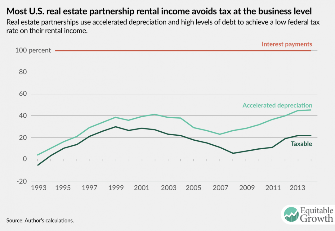
Statistics on the rental income of partnerships in the real estate industry provide a useful illustration of how accelerated depreciation and interest deductibility operate to shelter capital income from tax at the business level and thus generate low effective marginal tax rates. Moreover, as real estate partnerships account for more than $2 trillion of depreciable assets (judged at book value), these results are relevant for the broader economy.30
Real estate partnerships reported $524 billion in gross rents, $484 billion in rental expenses, and $2 billion in gains from the sale of rental property in 2014, the most recent year for which data are available. Net income from rental activities for tax purposes was thus $43 billion.31 Of the rental expenses, interest payments accounted for $114 billion and depreciation deductions for $109 billion.
Because depreciation for tax purposes differs from economic depreciation, it would not be appropriate to use the $43 billion in income reported on tax returns plus interest payments as an estimate of the economic income generated by the sector. Instead, estimating the economic income of these businesses requires an adjustment to the reported depreciation values. Using the ratio of economic depreciation to tax depreciation reported in the National Income and Product Accounts for sole proprietorships and partnerships to adjust the depreciation reported on real estate partnership tax returns yields an estimate of $59 billion for economic depreciation in the sector.32 This approximation suggests the economic income generated by rental partnerships—on behalf of equity owners and lenders—was about $208 billion, equal to the net income reported on tax returns plus interest and tax depreciation less economic depreciation. Thus, the taxable income reported from real estate activities was only 21 percent of the economic income generated by the sector.33 Of course, as partnerships are pass-through entities, the tax paid on the taxable share depends on the characteristics of the partners.
Figure 1 shows the same calculation for the years 1993 to 2014. Average net income at the business level for rental partnerships is only 16 percent of the economic income generated by these businesses over this period.
Figure 1
While interest payments reflect a permanent avoidance of business-level tax, accelerated depreciation allowances only change the timing of tax payments. Thus, for a specific investment project, an additional dollar of depreciation allowances today results in a dollar less of depreciation allowances in the future. But depending on the pattern of investment returns and asset sales over time, the aggregate taxable share of income for all partnerships could remain less than economic income less interest payments in all years.
Moreover, real estate partnership tax returns suggest that tax rates similar to those reported in this brief may overstate the tax paid on investments in that industry. The largest single source of income reported by these partnerships in many years is not rental income, but section 1231 gains. These gains are likely generated in large part by the sale of rental property, and the tax rates applied to such gains are often substantially lower than the rates that apply to rental income. The modeling underlying the estimates reported in this brief rules out the sale of business property and assumes that the tax rate applicable to business income is constant over time. Thus, if depreciation deductions are increased by a dollar today and reduced by a dollar in the future, then the tax savings today and the additional tax in the future are the same before discounting. If, instead, businesses benefit from depreciation deductions today at a higher tax rate and then sell assets later while facing a lower tax rate, accelerated depreciation can be worth more than the modeling assumes.
Finally, while this brief focuses on produced capital consisting of equipment, structures, inventories, and intangible assets, the rental industry relies to a substantial extent on land, which is available in relatively fixed quantity. Real estate partnerships report land equal to roughly one-third of the value of depreciable assets, judged at book value. A substantial fraction of the income reported by rental partnerships thus reflects returns on land rather than returns on produced capital. In fact, assuming debt financing of roughly 60 percent—a higher share than assumed in the tax rate estimates presented in this brief but not unreasonable given the estimates in Figure 1 above—the business-level effective marginal tax rate on structures would be about zero, and the effective marginal tax rate on land would be about 10 percent for both C corporations and pass-through businesses. These tax rates suggest that nearly all the rental income reported on real estate partnership returns is a return to land, excess returns, or labor income—not to investments in structures.
Implications for tax reform
Business-level federal effective marginal tax rates on capital income are quite low: 8 percent under current law and 13 percent if bonus depreciation expires. Rates are strongly negative for debt-financed investment, at negative-54 percent, and positive for equity-financed investment, at 21 percent. Moreover, other recent research suggests that the overwhelming majority of the corporate tax base consists of excess returns and labor income, not the risk-free return on produced capital.34
In light of these findings, the case for reductions in the statutory business tax rate as a means of spurring additional capital investment is weak. A reduction in the business tax rate would come at a very high cost, as it would apply to the entire business tax base, including excess returns and labor income, as well as to returns on investments made in the past.35 The impact on capital investment would be highly attenuated, as debt-financed investments face a negative rate at the business level, and thus a rate cut would increase the tax rate on such investments by reducing the value of the deductions they generate. Moreover, as lowering the cost of capital is the channel through which a reduced effective marginal tax rate can increase investment, deficit-financed tax cuts that increase the cost of capital can be actively counterproductive.
While the average rate is low, there is substantial variation in tax rates across asset types and financing arrangements. If 36 percent of each investment is financed with debt—the baseline assumption about the use of debt finance in this brief—then inventory investment is taxed at 28 percent, and intangible investment is taxed at a rate of negative-25 percent. Equipment is taxed at a near-zero rate, and structures are taxed at a rate of 13 percent. If, instead, 50 percent of investment in structures is financed with debt, then the effective marginal tax rate on such investment is only 6 percent. The tax rate that would apply to any real-world investment would almost certainly differ from any of these tax rates, as it would rely on financing and legal arrangements different from any of the scenarios presented.
A better approach to reform would therefore focus on reducing the disparities in tax rates across types of produced capital and across financing arrangements. This variation is largely driven by variation in the extent to which tax depreciation is accelerated relative to economic depreciation and variation in the use of debt finance. Well-designed reform should thus pursue a revenue-neutral or revenue-increasing reallocation of the current tax benefits for debt to equity that reduces the disparities in the tax rates on investments in different types of produced capital. Such a reallocation could also lower the tax rate on produced capital and increase the tax rate on land. These reforms would offer a more plausible path to economic growth than reductions in the statutory tax rates on business income.
Republicans in Congress and in the Trump administration have turned to tax reform, touting it as crucial for investment, job creation, and economic growth that will benefit American workers. While most policymakers agree that tax reform is overdue, true reform seems far less likely than poorly designed corporate tax cuts, and economic research shows that the results from such tax cuts are likely to be deeply disappointing to American workers. The benefits from these corporate tax cuts would accrue to corporate shareholders and senior managers—the same groups that have prospered the most in recent decades, while wages for middle-class Americans have stagnated.
If policymakers actually want to help American middle-class workers with tax cuts, they should simply direct those tax cuts to the taxes these workers pay. Income and payroll taxes are by far the dominant source of workers’ federal tax payments. There is no question that workers pay nearly all payroll and labor income taxes, including the portion of the payroll tax ostensibly paid by employers since workers pay for the employer portion of the payroll tax in the form of lower wages.
How would corporate tax cuts affect the middle class? For corporate tax cuts to benefit workers, the resulting increase in corporate after-tax profits would need to fuel new investments, those new investments would need to increase the productivity of labor, and the higher productivity would need to boost wages. But why rely on indirect mechanisms to help workers when we have far more direct tools? If the aim is to help workers, then policymakers should go straight to the taxes that fall on them. Workers would get nearly 100 percent of payroll and labor income tax cuts.
Research shows that corporate tax cuts are far more likely to end up in the hands of those at the top of the income distribution. All major models from the Joint Committee on Taxation, the Congressional Budget Office, the U.S. Department of Treasury, and the nonpartisan Tax Policy Center put the vast majority of the corporate tax burden on capital or shareholders. And there is little to no empirical evidence that corporate tax cuts increase investment and wages across countries; research suggesting as much has rarely found a place in peer-reviewed publications, and early implausible results have been subsequently questioned or overturned.
Further, much of the U.S. corporate tax base at present is excess profits, which are profits above the normal level accruing due to intangible sources of economic value and market power. U.S. Treasury economists now calculate that three-quarters of the corporate tax base is excess profits, often in the hands of very few superstar companies. Giving a tax cut to this part of the tax base just makes excess profits even larger, without stimulating capital investment or wages.
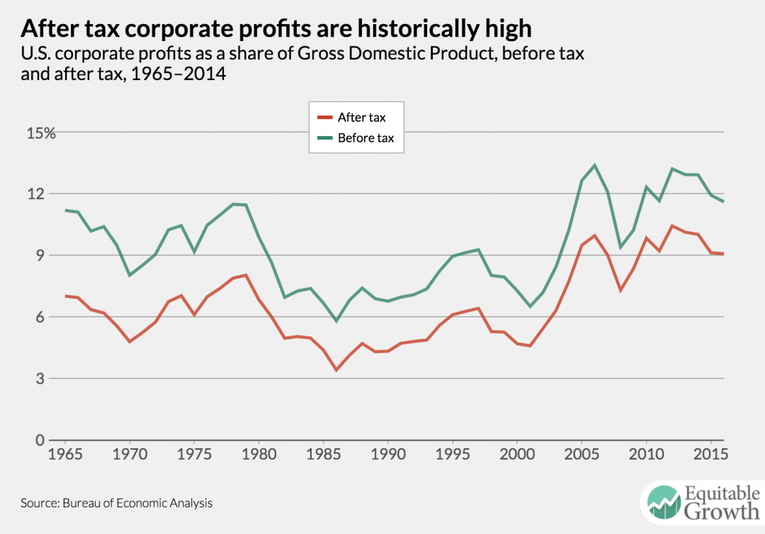
If burgeoning corporate after-tax profits were the key to investment and wage growth, then the previous 15 years should have been a paradise of wage growth, as after-tax profits in recent years have been about 50 percent higher than in decades prior (as a share of Gross Domestic Product), and higher than at any point in the past half-century. (See Figure 1.)
Figure 1
Are policymakers really to believe that low after-tax profits are the key economic problem that tax reform should address? Those arguing for corporate tax cuts typically cloak their arguments under the guise of competitiveness. But this is nonsense. Our multinational companies are the most competitive on the planet. The United States has a disproportionate share of the Forbes 2000 list of global companies, and after-tax profits are at record levels. Further, our multinational companies are so skillful at exploiting loopholes to lower their tax bills that they often achieve effective tax rates in the single digits. Business tax reform should not lower tax collections from the country’s corporations—collections that are already 1 percent of GDP lower than corporate tax collections in other countries.
To be clear, there is a pressing need for corporate tax reform. Such reform could lower headline rates somewhat if policymakers were serious about protecting the corporate tax. Evidence suggests that the U.S. government is probably losing more than $100 billion each year due to corporate profit shifting to tax havens, and a similar amount of revenue is being lost as business activity moves into pass-through form. This leaves a lot of room for true tax reform to simultaneously close loopholes and lower rates. But the rates that have been suggested—rates as low as 15 percent or 20 percent—would not deliver substantial economic benefits for the middle class and would instead result in huge revenue losses for the federal government and a much lighter tax burden for those at the top of the income distribution. Further, there is no indication that these proposals will be serious about corporate tax-base protection.
So far, tax cuts seem to be far more important to Republican policymakers and the Trump administration than tax reform, and the planned tax cuts are heavily skewed toward those at the top at the expense of future generations of taxpayers. To help middle-class workers, give them the tax cuts, and keep business tax reform—and tax reform as a whole—at least revenue neutral.
— Kimberly Clausing is the Thormund A. Miller and Walter Mintz Professor of Economics at Reed College.
The release today of the U.S. Census Bureau’s annual report on income and poverty underscores why better official measures of economic inequality are sorely needed. Official measures released by the Census Bureau and based on the Current Population Survey underreport the level and trend of inequality. The federal government should follow the lead of academic economists who are taking a more rigorous approach to measuring income—an approach that has allowed them to detect rapid increases in the income of very high earners that the federal government’s statistics have missed.
To be sure, the Census Bureau’s annual report for 2016 is one of the most high-profile official products of the federal government that attempts to quantify economic inequality. These estimates are calculated using the Annual Social and Economic Supplement of the Census’ Current Population Survey. The CPS is one of the best sources of economic data available on the earnings of U.S. workers, but it has limitations and cannot be relied on to estimate incomes at the very top of the income distribution.
According to today’s data, the share of income earned by the poorest 20 percent of Americans declined from about 4 percent of the total in 1967 to 3.1 percent in 2016. The middle 20 percent clearly lost ground over the same period of time. And there was a relatively modest rise in the share of income taken by the richest 5 percent of the population: from 17.2 percent in 1967 to 22.6 percent in 2016 (see Figure 1).
Figure 1
But these estimates of inequality by the Census Bureau do not tell the full story. Another dataset compiled by the academic team of economists Thomas Piketty at the Paris School of Economics and Emmanuel Saez and Gabriel Zucman at the University of California, Berkeley finds that the share of income garnered by the top 5 percent was much higher to begin with, 25.7 percent in 1967, and climbed more sharply to 36.1 percent of all income by 2014. Their estimates are based on a dataset they created called Distributional National Accounts. (See Figure 2.)
Figure 2
The Distributional National Accounts data suggest a much more unequal United States and a far steeper rise in inequality over the past four decades. Unfortunately, these data are closer to the truth than the Census estimates because they incorporate higher-quality administrative data and include more sources of income. It is especially unfortunate because the Census Bureau’s report is one of the few official data sources for tracking inequality, but for methodological reasons—most of which are outside the agency’s control—this official indicator is missing important trends.
Official U.S. economic measurement must improve
Without accurate measurement, policymakers cannot determine whether the laws and regulations they enact result in more broad-based economic prosperity. The three economists who developed the Distributional National Accounts prototype measurement point the way forward. Although there are many differences between their estimates and official estimates from the Census Bureau, two factors explain most of the discrepancy. First, the academic team uses administrative data to supplement the CPS survey data. Second, the Distributional National Accounts measurement uses a more complete definition of income. Here’s why both factors are so important to improving the measurement of the U.S. economy.
Survey data versus administrative data
The Census Bureau’s inequality estimates are based on data from the Current Population Survey. The Annual Social and Economic Supplement to the survey, conducted every March, provides economic data that is widely used by researchers, policymakers, and pundits. The CPS is a high-quality survey that goes out to more than 75,000 households, but even with such a relatively large sample size, it is difficult to capture the incomes of the truly rich, as they represent a tiny slice of the population and may be less likely than others to respond to a survey. As a result, measures of income in the CPS become less reliable as you look at higher and higher income slices of the U.S. population.
The academic team behind Distributional National Accounts addresses this weakness in the CPS by incorporating administrative tax data from the U.S. Internal Revenue Service. This gives them access to actual income reported to the IRS for every filer in the country. They can therefore construct more accurate estimates of income for top earners, all the way into the top 0.001 percent. This turns out to be extremely important because the fortunes of the merely rich and the truly rich have diverged considerably.
How much has the share of national income changed for the top 10 percent, the top 1 percent, and the top 0.1 percent of earners between 1967 and the end of 2016? The top 10 percent experienced an increase of a mere 15 percent in their share of total economic income, while the top 1 percent gained 37 percent and the richest 0.1 percent of earners more than doubled their share of total income, from 4.4 percent to 9.3 percent—a staggering 114 percent increase. (See Figure 3.)
Figure 3
The Census Bureau, relying on considerably less comprehensive data from the CPS, is only able to document the top 5 percent of income earners, and we know from the tax data that the CPS considerably underestimates income in that segment. Without incorporating administrative data, a full accounting of inequality in the United States is impossible. Importantly, this is not the Census Bureau’s fault. They do not have access to the full tax data that Piketty, Saez, and Zucman do, though they do have access to a more limited extract with less income detail. Nor is the IRS arbitrarily withholding data: U.S. law puts strict limits on how tax return data can be shared. If the federal government is ever to produce strong inequality statistics, these limits may have to be revisited in ways that preserve confidentiality while allowing improved measures of economic outcomes.
Measures of income
A second way in which the Census Bureau estimates miss the mark is in their chosen definition of income. The agency tracks money income, a measure that includes most sources of raw income that an earner might accrue before taxes are levied. It doesn’t include nonmonetary compensation such as the value of employer-provided health care. Finally, the agency takes a mixed approach to government transfers. Some are included as income such as Social Security income, while noncash benefits are excluded such as supplemental nutrition assistance.
Once again, the approach taken by Piketty, Saez, and Zucman is instructive. There are two significant distinctions in how Distributional National Accounts measure income. First, they peg their estimates to the National Income and Product Accounts. These accounts, produced by the U.S. Bureau of Economic Analysis, track the total economic output of goods and services in the United States to produce Gross Domestic Product. Add the income of every individual in the Distributional National Accounts dataset together, and it matches income concepts in the National Income and Product Accounts.
This matching requires the academic team to make some decisions that may seem odd at first glance. The three economists take all government spending on public education, for example, and allot it to individuals in the dataset. The average person may not think about this money as being part of their income, but it is a government benefit that subsidizes the income of those with children; for those without children, it helps to create a more educated and hopefully better society. Pegging the dataset to the National Income and Product Accounts ensures that all income is accounted for and gives a more complete picture of how government policy impacts inequality.
Second, Piketty, Saez, and Zucman provide measures for income before and after government taxes and transfers. Measuring inequality before and after government taxes and investments in social welfare programs is an important part of understanding how policy affects inequality. Among the wealthiest economies in the world, the United States is not very notable for its pre-tax and transfer level of inequality. France and Germany, for example, have similar levels of inequality, but the United States does much less redistribution with its tax code and social welfare programs. The upshot: The French and German economies are much less unequal after government programs are accounted for than the U.S. economy.
How do government taxes and transfers affect the share of income held by, say, the top 5 percent in the United States? The gap between pre-tax and post-taxes and transfers income has been widening since the early 1990s, and currently this gap accounts for about a 7 percentage point difference for this income group. (See Figure 4.)
Figure 4
This before-and-after information is absolutely necessary if policymakers are to understand how their policies affect economic inequality. If there is only one measure of inequality, it may be difficult to deduce whether fluctuations are caused by policy or some exogenous factor.
Today’s data release by the U.S. Census Bureau is an important product because it represents one of the nation’s few official measures of inequality. But it is insufficient if we are to truly understand how inequality has changed and how it affects today’s economy. Legislators and employees of statistical agencies alike should pursue ways of improving our data infrastructure for tracking inequality.
It is increasingly apparent that many policymakers and commentators believe that business tax reform means reducing the statutory corporate tax rate. This fixation on the corporate tax rate is unfortunate and misguided. Business tax reform should be primarily about the tax base, not the tax rate. Treating the statutory rate as the key element of reform will inevitably result in a more expensive, more regressive, and less economically beneficial (if not actively harmful) reform than one that focuses on the tax base. By focusing on the base, it is possible to design reforms that achieve a given set of economic objectives at a far more modest cost. Focusing on the base therefore also makes it much easier to meet the minimum standard that tax reform should not decrease government revenues.
The focus on the rate is apparent in the evolution of public statements about tax reform from congressional Republicans and Trump administration officials. Modifications of the tax base were an important part of the blueprint for tax reform put out by Republicans in the House of Representatives in 2016. The blueprint contained three major proposed changes to the corporate tax: a reduction in the statutory rate; full expensing of capital investment combined with repeal of interest deductibility; and the imposition of a border adjustment that would tax imports and rebate tax on exports. But the joint statement on tax reform from six leading Republicans representing both Congress and the administration at the end of July expressed less enthusiasm for expensing and rejected outright the border adjustment, leaving the reduction in the statutory corporate rate the only element unscathed. More recently, National Economic Council Director Gary Cohn reiterated the administration’s focus on the statutory corporate rate, saying that the administration will seek the lowest statutory rate possible.
Recent research indicates that the overwhelming majority of the corporate tax base consists of excess returns, meaning returns above the risk-free rate such as those due to monopoly pricing power, and income attributable to labor that was not paid out as wages. Cutting the corporate tax rate is inefficient and regressive because these types of income are relatively efficient to tax and accrue to business owners, who are disproportionately high-income and high-wealth.
Consistent with these findings, the corporate-level tax rate on the marginal investment—the tax rate paid on a hypothetical investment in tangible or intangible capital that yields the minimum return necessary to attract financing in capital markets—is far lower than the statutory tax rate: only 6 percent, according to recent estimates from the Congressional Research Service. This rate is lower than the statutory tax rate due to provisions of the corporate tax system such as accelerated depreciation and interest deductibility that allow a substantial portion of the return on corporate investment to avoid corporate tax. Proposals for business tax reform that focus on the base rather than the rate can achieve a much more attractive combination of benefits and costs than reforms that focus on cutting the statutory tax rate because they aim to keep as large a share of excess returns and disguised labor income in the tax base as possible.
The advantages of focusing on the tax base rather than the corporate tax rate are usefully illustrated by two proposals recently put forward by the tax policy community, both of which achieve the economic objectives of their proponents at far lower cost than reducing the statutory rate in isolation.
First, consider the destination-based cash flow tax. Adopting this proposed tax would effectively repeal the corporate income tax without reducing the statutory tax rate at all. The proposal would change the tax base—allowing full expensing of capital investment, repealing interest deductibility, taxing imports, and rebating tax on exports—in such a way that it would convert the corporate income tax into another type of tax entirely: an approximation to the business cash flow tax that is part of a consumption tax system. In other words, even if one adopts the view that corporate income taxes are uniquely distortionary and should be eliminated, it is possible to do so without reducing the rate. (The policies listed above do not yield a pure destination-based cash flow tax, as they would still tax certain corporate financial income, including interest, dividends, and capital gains.)
Next, consider the proposal for corporate tax reform put forward by Eric Toder at the Tax Policy Center and Alan Viard at the American Enterprise Institute. This proposal would reduce the corporate tax rate to 15 percent while taxing investors on the change in the value of their shares in publicly traded companies on an annual basis (and providing credit for corporate taxes paid to taxable investors). The proposal also would impose tax on interest income received by nonprofit organizations and by individuals in their retirement accounts, such as 401(k)s and individual retirement accounts.
The proposal by Toder and Viard includes a reduction in the statutory rate, but it is more usefully understood as a redefinition and reallocation of the tax base across entities. By taxing investors on the change in the value of their shares, a substantial fraction of the corporate tax base is effectively shifted from the corporate level to the investor level. The new taxes applied to certain interest payments offset the exclusion of interest payments from the corporate tax base, thus achieving a more consistent treatment of investments financed in different ways. The major changes in the tax base in this proposal are the implicit partial exclusion of corporate income attributable to foreign investors and the use of market valuations rather than measuring income directly.
The common theme of these two proposals is a reform that modifies the tax base to achieve clear economic objectives at a more modest cost than simply cutting the corporate tax rate. The destination-based cash flow tax proposal shows that it is possible to completely repeal the corporate income tax in an economic sense without reducing the statutory corporate tax rate to zero. The Toder-Viard proposal highlights that full or partial integration proposals can achieve similar economic aims by shifting the tax base between firm-level taxes and investor-level taxes, provided that the investor-level taxes are appropriately reformed.
Estimates from the Tax Policy Center suggest that both the Toder-Viard proposal and the not-quite-pure destination-based cash flow tax could be implemented on a roughly revenue-neutral basis in the first decade, including the cost of providing expensing for noncorporate businesses in the cost of the latter proposal. Although both proposals have important weaknesses, either one would offer a far more attractive combination of costs and benefits than a simple reduction in the statutory corporate tax rate.
A key implication of the existence of these proposals is that simple arguments against corporate income taxation or capital taxation, even if true, are inadequate to make the case for statutory corporate rate cuts as the centerpiece of reform. Arguing for statutory rate cuts requires first rejecting superior and far cheaper policy alternatives.
Indeed, the variants of these two plans that have achieved political traction highlight the problems of focusing on the statutory tax rate. The House Republican blueprint draws heavily from the destination-based cash flow tax but adds a large cut in the statutory corporate tax rate. This rate cut would come at great cost, would be a key contributor to the higher federal budget deficits that would cause the blueprint to harm economic growth, would provide little or no economic benefit even if financed by other tax increases or spending cuts, and would be severely regressive. In effect, the blueprint shifts the United States toward a consumption tax but then adds a partial exemption for consumption by business owners (via the rate cut) with no justification.
Similarly, there has been some congressional interest in increasing tax rates on capital gains and dividends as a potential offset for statutory corporate rate cuts, but little apparent interest in the more fundamental reforms to taxation at the investor level that are core to the Toder-Viard proposal. The focus on offsets for a statutory rate cut rather than a focus on the appropriate base for taxation ultimately undermines any economic merits the proposal might otherwise have.
Regardless of one’s views on the relative merits of consumption taxation and income taxation, on the economic and fiscal costs of the erosion of the corporate tax base, or on the harm resulting from corporate inversions, business tax reform should be about reforming the tax base, not cutting the rate. Cutting the rate is an expensive and regressive substitute for other superior reforms.
Many arguments for reducing the corporate tax rate are in large part arguments for increased reliance on consumption taxes. Plausible tax legislation, however, looks quite different from reforms that would move the United States toward a consumption tax. (In the interest of disclosure, this author is not an advocate of converting the income tax into a consumption tax.) The idealized consumption tax would tax labor and excess returns while exempting from tax the risk-free return to capital. Thus, relative to current law, legislation would focus on exempting the risk-free return and leave the taxation of excess returns unaffected to the extent possible. But with the apparent focus in Congress and within the Trump administration on reducing the statutory corporate tax rate, plausible tax legislation is more likely to reverse those outcomes, reducing taxes on excess returns to the maximum extent possible and leaving the taxation of risk-free returns relatively unaffected. This approach is not the path to equitable growth.
Children born into poor and wealthy families alike should have an equal chance of achieving their dreams. But this is not the reality in practice. The income of a child’s parents is strongly correlated with the child’s life outcomes—such as educational attainment, occupational choice, or earnings—in adulthood. Opportunity is far from equal.
Recent research shows that the strength of the association between the child’s parents’ income and her own adult income—a useful measure of inequality of opportunity—varies a great deal between different places across the United States. In some areas, such as Salt Lake City and Los Angeles, the intergenerational association is small, which means the chances for children from low-income families to get ahead are close to those of children from high-income families, so opportunity is relatively equal.
In other areas, however, such as Cincinnati and Memphis, intergenerational associations are strong, meaning differences in life outcomes between children from low-income versus high-income families are large and that opportunity is far from equally distributed. Children from low-income families are less likely to do better than their parents, while children of high-income parents will stay in the upper income brackets.
What explains the geographic variation in this intergenerational transmission of economic status? What is going right in Los Angeles and Salt Lake City but going wrong in Cincinnati and Memphis? A natural hypothesis is that these differences have to do with the quality of the local schools. Schools should be an engine of economic mobility, allowing bright, hardworking children to advance regardless of their family backgrounds. But schools are themselves often unequally distributed, and many schools serving poor children are poorly funded and low-performing.
So perhaps some low-transmission, high-economic-equality cities such as Salt Lake City and Los Angeles simply have better, more equal school systems that produce better and more equal educational outcomes and thus more equal incomes as adults. Or perhaps the differences have nothing to do with schools and instead relate to differences in labor markets in these cities—perhaps when job opportunities are more plentiful and pay is more equal, it does not matter as much whether a child had access to good schools.
In a recent paper, I assess the contributions of education and labor markets to differences across regional labor markets—commuting zones—in the United States in the intergenerational transmission of economic status. To do this, I ask whether parental income matters more for children’s educational outcomes, such as test scores and college completion, in local areas where there is stronger transmission of parental income to children’s incomes, as would be expected if the school system were a key link in this transmission.
I find that there is a great deal of variation in educational transmission across the country. Some areas do much better than others at producing closer-to-equal test scores for children from poor and rich families. Yet areas with small test-score gaps do not have lower-than-average income transmission. In other words, differences in access to high-quality elementary and secondary schools are not a key channel driving the strength of the association between parents’ incomes and their children’s incomes when they reach adulthood.
There is a bit more evidence that higher education is an important part of the story. Gaps in college enrollment and graduation are associated with intergenerational income transmission, though even here, the association is too small to account for much of the variation between regions in income transmission.
The upshot: There is little evidence that differences in the quality of primary, secondary, or postsecondary schools, or in the distribution of access to good schools, are a key mechanism driving variation in intergenerational mobility. The evidence instead points toward other factors influencing income inequality. In particular, labor markets seem to be quite important. Even when children’s test scores and educational attainment are held constant, children from poor families have higher adult earnings when they grow up in low-transmission (greater-opportunity) areas than when they are from low-opportunity, high-transmission areas. This is in part because the high-transmission areas have unusually large returns to human capital, or stronger relationships between education and earnings. Children from wealthy families do better in school than children from poor families everywhere, so a labor market that puts inordinate weight on skill will be unusually favorable to the wealthy children.
Marriage patterns also seem to matter. In cities and regions where income transmission is weaker, the “marriage gap” between those in their mid-20s from low- and high-income families is much smaller, implying that children from low-income families are more likely to have spouses contributing toward the family budget.
Together, differences in labor markets and marriage patterns account for the great majority of variation in intergenerational mobility across cities and regions in the United States. Variation in relative skill accumulation—the only portion plausibly related to schools—accounts for only 12 percent of the differences between high- and low-opportunity areas, with the rest due to marriage patterns (about one-third) and differences in labor market outcomes operating through channels other than skill accumulation, such as the return to skill in the labor market, discrimination, or referral networks that offer advantaged children a leg up in the job market (about half). (See Figure 1.)
Figure 1
Understanding better how policymakers can promote equality of opportunity in education as well as in the economy overall should remain a top priority. Educational quality is certainly a key tool to improve opportunity, yet my research indicates that it is far from the whole story. The educational system plays only a small role in explaining differences between high- and low-opportunity areas. Labor market institutions—such as minimum wages, the ability to form and join unions, the career structures of local industries, and other determinants of earnings inequality—are likely to play much larger roles and are also likely to be more powerful levers with which to promote equality of opportunity.
The principle of equal access to the pursuit of happiness is deeply rooted in American history and society. We have never accomplished it, but it remains our country’s highest aspiration. The best measure of the progress we have made toward this goal is the extent to which the circumstances of a child’s birth do or do not predict his or her life outcomes. By this measure, as by others, we have very far to travel. To do better, we need to examine all of the different ways that our society and economy work to erect hurdles in front of children from disadvantaged families—whether those hurdles are limiting access to educational opportunity or ensuring that the children will do worse in the labor market than their more advantaged peers even if they do well in school.
—Jesse Rothstein is a professor of public policy and economics at the University of California, Berkeley, and director of the Institute for Research on Labor and Employment at the University of California, Berkeley.