A snapshot of the long-term impacts of universal pre-k in Minnesota

If the United States were to invest in a public, voluntary, high-quality universal prekindergarten program starting in 2016 and fully phased in by 2017, what would the long-term impacts be for ? Our study looks to quantify the long-term benefits and costs of investing in a high-quality universal prekindergarten program available to all 3- and 4-year-olds across the United States. Use the data and interactives below to explore how a universal prekindergarten program would affect .

Who would participate?

Currently, in , percent of 3- and 4-year-olds ( children) participate in state-sponsored prekindergarten. Unfortunately, the quality of these programs varies significantly, which means that preschoolers do not always experience the same benefits or long-term effects. If a universal prekindergarten program were enacted in 2016 and fully phased in by 2017, percent of 3- and 4-year-olds ( children) would be enrolled in public prekindergarten, benefiting from a high-quality early childhood education.

What are the benefits of a universal prekindergarten program?

High-quality prekindergarten education can generate significant long-run benefits for participating children, their families, and even other non-participants. Longitudinal studies have shown, for example, that aside from improved educational achievement, children who have attended a prekindergarten program have spent less time in special education and had lower grade retention rates. These children also experience less child maltreatment and reduced crime, smoking, and depression rates over the course of their lives. In addition, both participating children and their parents have higher projected earnings, which subsequently increases government tax revenue.

If a universal prekindergarten program were to start in the United States in 2016, would see more than $ million in total benefits in 2050, amounting to savings of $ per capita that year. Here’s how these total benefits break down:

  • $ per person is attributed to savings to government.
  • $ per person comes from increased compensation.
  • The remaining $ per person is accounted for by savings to each individual from better health and less crime.

What are the costs?

Currently, spends $ per capita per year on preschool programs, special education services, and Head Start. In 2017, when a universal prekindergarten program is fully phased in, it would take an investment of $ more per capita per year to maintain a high-quality prekindergarten program.

There are three main costs associated with a high-quality universal prekindergarten program: the cost of the program, increased high school attendance, and increased college attendance. The program itself is based on Chicago’s comprehensive high-quality Child-Parent Center half-day program, so the costs take into account the multitude of services that are provided at the Child-Parent Center offset by the current spending on similar early childhood education programs as to not double-count expenditures. Because studies have shown that students who attend prekindergarten have higher high school completion rates and are more likely to attend college, these usage costs are also factored into the total cost of a universal prekindergarten program.

In 2050, these costs add up to an additional $ million, or $ per capita in . $ per capita is attributed to program costs, $ comes from increased high school usage per person, and the remaining $ per person is accounted for by increased college attendance.

How do the benefits compare to the costs?

If a high-quality universal prekindergarten program were to start in the United States in 2016 and be fully phased in by the end of 2017, the program would require a total of $ million in taxpayer dollars. Over time, the cost would eventually grow to include the cost of additional high school and college attendance. And by 2050, there would be more than $ million in total benefits compared to merely $ million in total costs, yielding net benefits of $ million. By 2050, for every dollar invested in a universal program, there would be $ in returns.

To see the national numbers, return to the full report.

A snapshot of the long-term impacts of universal pre-k in California

If the United States were to invest in a public, voluntary, high-quality universal prekindergarten program starting in 2016 and fully phased in by 2017, what would the long-term impacts be for ? Our study looks to quantify the long-term benefits and costs of investing in a high-quality universal prekindergarten program available to all 3- and 4-year-olds across the United States. Use the data and interactives below to explore how a universal prekindergarten program would affect .

Who would participate?

Currently, in , percent of 3- and 4-year-olds ( children) participate in state-sponsored prekindergarten. Unfortunately, the quality of these programs varies significantly, which means that preschoolers do not always experience the same benefits or long-term effects. If a universal prekindergarten program were enacted in 2016 and fully phased in by 2017, percent of 3- and 4-year-olds ( children) would be enrolled in public prekindergarten, benefiting from a high-quality early childhood education.

What are the benefits of a universal prekindergarten program?

High-quality prekindergarten education can generate significant long-run benefits for participating children, their families, and even other non-participants. Longitudinal studies have shown, for example, that aside from improved educational achievement, children who have attended a prekindergarten program have spent less time in special education and had lower grade retention rates. These children also experience less child maltreatment and reduced crime, smoking, and depression rates over the course of their lives. In addition, both participating children and their parents have higher projected earnings, which subsequently increases government tax revenue.

If a universal prekindergarten program were to start in the United States in 2016, would see more than $ million in total benefits in 2050, amounting to savings of $ per capita that year. Here’s how these total benefits break down:

  • $ per person is attributed to savings to government.
  • $ per person comes from increased compensation.
  • The remaining $ per person is accounted for by savings to each individual from better health and less crime.

What are the costs?

Currently, spends $ per capita per year on preschool programs, special education services, and Head Start. In 2017, when a universal prekindergarten program is fully phased in, it would take an investment of $ more per capita per year to maintain a high-quality prekindergarten program.

There are three main costs associated with a high-quality universal prekindergarten program: the cost of the program, increased high school attendance, and increased college attendance. The program itself is based on Chicago’s comprehensive high-quality Child-Parent Center half-day program, so the costs take into account the multitude of services that are provided at the Child-Parent Center offset by the current spending on similar early childhood education programs as to not double-count expenditures. Because studies have shown that students who attend prekindergarten have higher high school completion rates and are more likely to attend college, these usage costs are also factored into the total cost of a universal prekindergarten program.

In 2050, these costs add up to an additional $ million, or $ per capita in . $ per capita is attributed to program costs, $ comes from increased high school usage per person, and the remaining $ per person is accounted for by increased college attendance.

How do the benefits compare to the costs?

If a high-quality universal prekindergarten program were to start in the United States in 2016 and be fully phased in by the end of 2017, the program would require a total of $ million in taxpayer dollars. Over time, the cost would eventually grow to include the cost of additional high school and college attendance. And by 2050, there would be more than $ million in total benefits compared to merely $ million in total costs, yielding net benefits of $ million. By 2050, for every dollar invested in a universal program, there would be $ in returns.

To see the national numbers, return to the full report.

A snapshot of the long-term impacts of universal pre-k in Washington, D.C.

If the United States were to invest in a public, voluntary, high-quality universal prekindergarten program starting in 2016 and fully phased in by 2017, what would the long-term impacts be for ? Our study looks to quantify the long-term benefits and costs of investing in a high-quality universal prekindergarten program available to all 3- and 4-year-olds across the United States. Use the data and interactives below to explore how a universal prekindergarten program would affect .

Who would participate?

Currently, in , percent of 3- and 4-year-olds ( children) participate in state-sponsored prekindergarten. Unfortunately, the quality of these programs varies significantly, which means that preschoolers do not always experience the same benefits or long-term effects. If a universal prekindergarten program were enacted in 2016 and fully phased in by 2017, percent of 3- and 4-year-olds ( children) would be enrolled in public prekindergarten, benefiting from a high-quality early childhood education.

What are the benefits of a universal prekindergarten program?

High-quality prekindergarten education can generate significant long-run benefits for participating children, their families, and even other non-participants. Longitudinal studies have shown, for example, that aside from improved educational achievement, children who have attended a prekindergarten program have spent less time in special education and had lower grade retention rates. These children also experience less child maltreatment and reduced crime, smoking, and depression rates over the course of their lives. In addition, both participating children and their parents have higher projected earnings, which subsequently increases government tax revenue.

If a universal prekindergarten program were to start in the United States in 2016, would see more than $ million in total benefits in 2050, amounting to savings of $ per capita that year. Here’s how these total benefits break down:

  • $ per person is attributed to savings to government.
  • $ per person comes from increased compensation.
  • The remaining $ per person is accounted for by savings to each individual from better health and less crime.

What are the costs?

In 2050, these costs add up to an additional $ million, or $ per capita in . $ per capita is attributed to program costs, $ comes from increased high school usage per person, and the remaining $ per person is accounted for by increased college attendance.

There are three main costs associated with a high-quality universal prekindergarten program: the cost of the program, increased high school attendance, and increased college attendance. The program itself is based on Chicago’s comprehensive high-quality Child-Parent Center half-day program, so the costs take into account the multitude of services that are provided at the Child-Parent Center offset by the current spending on similar early childhood education programs as to not double-count expenditures. Because studies have shown that students who attend prekindergarten have higher high school completion rates and are more likely to attend college, these usage costs are also factored into the total cost of a universal prekindergarten program.

In 2050, these costs add up to $ million, or $ per capita in . $ per capita is attributed to program costs, $ comes from increased high school usage per person, and the remaining $ per person is accounted for by increased college attendance.

How do the benefits compare to the costs?

If a high-quality universal prekindergarten program were to start in the United States in 2016 and be fully phased in by the end of 2017, the program would require a total of $ million in taxpayer dollars. Over time, the cost would eventually grow to include the cost of additional high school and college attendance. And by 2050, there would be more than $ million in total benefits compared to merely $ million in total costs, yielding net benefits of $ million. By 2050, for every dollar invested in a universal program, there would be $ in returns.

To see the national numbers, return to the full report.

A snapshot of the long-term impacts of universal pre-k in Utah

If the United States were to invest in a public, voluntary, high-quality universal prekindergarten program starting in 2016 and fully phased in by 2017, what would the long-term impacts be for ? Our study looks to quantify the long-term benefits and costs of investing in a high-quality universal prekindergarten program available to all 3- and 4-year-olds across the United States. Use the data and interactives below to explore how a universal prekindergarten program would affect .

Who would participate?

Currently, in , percent of 3- and 4-year-olds ( children) participate in state-sponsored prekindergarten. Unfortunately, the quality of these programs varies significantly, which means that preschoolers do not always experience the same benefits or long-term effects. If a universal prekindergarten program were enacted in 2016 and fully phased in by 2017, percent of 3- and 4-year-olds ( children) would be enrolled in public prekindergarten, benefiting from a high-quality early childhood education.

What are the benefits of a universal prekindergarten program?

High-quality prekindergarten education can generate significant long-run benefits for participating children, their families, and even other non-participants. Longitudinal studies have shown, for example, that aside from improved educational achievement, children who have attended a prekindergarten program have spent less time in special education and had lower grade retention rates. These children also experience less child maltreatment and reduced crime, smoking, and depression rates over the course of their lives. In addition, both participating children and their parents have higher projected earnings, which subsequently increases government tax revenue.

If a universal prekindergarten program were to start in the United States in 2016, would see more than $ million in total benefits in 2050, amounting to savings of $ per capita that year. Here’s how these total benefits break down:

  • $ per person is attributed to savings to government.
  • $ per person comes from increased compensation.
  • The remaining $ per person is accounted for by savings to each individual from better health and less crime.

What are the costs?

Currently, spends $ per capita per year on preschool programs, special education services, and Head Start. In 2017, when a universal prekindergarten program is fully phased in, it would take an investment of $ more per capita per year to maintain a high-quality prekindergarten program.

There are three main costs associated with a high-quality universal prekindergarten program: the cost of the program, increased high school attendance, and increased college attendance. The program itself is based on Chicago’s comprehensive high-quality Child-Parent Center half-day program, so the costs take into account the multitude of services that are provided at the Child-Parent Center offset by the current spending on similar early childhood education programs as to not double-count expenditures. Because studies have shown that students who attend prekindergarten have higher high school completion rates and are more likely to attend college, these usage costs are also factored into the total cost of a universal prekindergarten program.

In 2050, these costs add up to an additional $ million, or $ per capita in . $ per capita is attributed to program costs, $ comes from increased high school usage per person, and the remaining $ per person is accounted for by increased college attendance.

How do the benefits compare to the costs?

If a high-quality universal prekindergarten program were to start in the United States in 2016 and be fully phased in by the end of 2017, the program would require a total of $ million in taxpayer dollars. Over time, the cost would eventually grow to include the cost of additional high school and college attendance. And by 2050, there would be more than $ million in total benefits compared to merely $ million in total costs, yielding net benefits of $ million. By 2050, for every dollar invested in a universal program, there would be $ in returns.

To see the national numbers, return to the full report.

An introduction to the geography of student debt

Today, the Washington Center for Equitable Growth, with Generation Progress and Higher Ed, Not Debt, released its interactive, Mapping Student Debt, which compares the geographic distribution of average household student loan balances and average loan delinquency to median income across the United States and within metropolitan areas. The stark patterns of student debt across zip codes enable us to begin to analyze the role that debt plays in people’s lives and the larger economy.

Delinquency and income

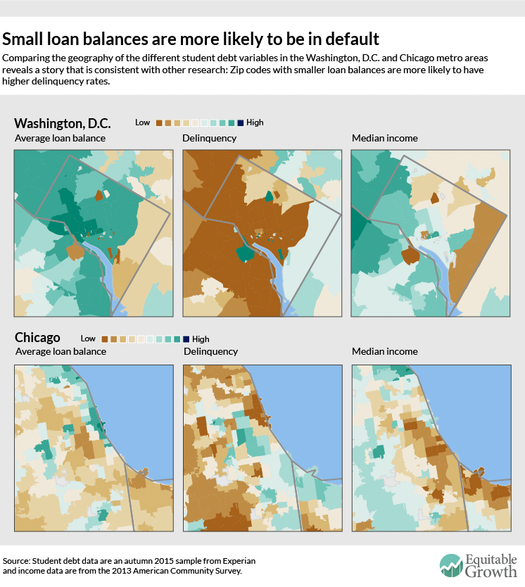
One element of the student debt story that has already been explored is that borrowers with the lowest student loan balances are the most likely to default because they are also the ones likely face the worst prospects in the labor market. Our analysis using the data displayed in the interactive map is consistent with these findings.

The geography of student debt is very different than the geography of delinquency. Take the Washington, D.C. metro region. In zip codes with high average loan balances (western and central Washington, D.C.), delinquency rates are lower. Within the District of Columbia, median income is highest in these parts of the city. Similar results–low delinquency rates in high-debt areas–can be seen for Chicago, as well. (See Figure 1.)

Figure 1

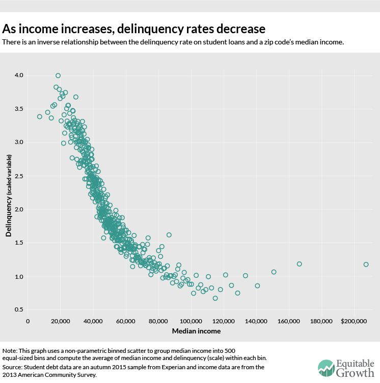
For the country as a whole, there’s an inverse relationship between zip code income and delinquency rates. As the median income in a zip code increases, the delinquency rate decreases, corroborating findings that low-income borrowers are the most likely to default on their loan repayments. (See Figure 2.)

Figure 2

What explains this relationship? There appear to be two possible, and mutually consistent, theories. First, although graduate students take out the largest student loans, they are able to carry large debt burdens thanks to their higher salaries post-graduation. One study of student loans by institution type reports a three-year cohort default rate for graduate-only institutions of 2 percent to 3 percent.* Second, the rise in the number of students borrowing relatively small amounts for for-profit colleges has augmented the cumulative debt load, but because these borrowers face poor labor market outcomes and lower earnings upon graduation (if they do in fact graduate), their delinquency rates are much higher. This is further complicated by the fact that these for-profit college attendees generally come from lower-income families who may not be able to help with loan repayments.

The inverse relationship between delinquency and income is not surprising, especially when considering that problems of credit access have disproportionately affected poor and minority populations in the past. In the 1930s, for example, the government-sanctioned Home Owner’s Loan Corporation labeled maps of American cities by each neighborhood’s worthiness for mortgage lending. Neighborhoods outlined in red were considered the least worthy, purposefully coinciding with their black and poor white populations. Banks and insurance agencies also adopted these discriminatory “redlining” practices, further cutting off communities from the essential capital that is needed to develop neighborhoods and invest in sustainable infrastructure. Though redlining was outlawed in the 1960s, its pernicious effects still persist, as seen in Figure 2 as well as in maps of the subprime mortgage crisis that began in 2006.

It might seem counterintuitive that lack of access to credit results in delinquency—seemingly a problem of “too much debt.” But in fact, lack of access to credit and delinquency are two sides of the same coin. Nearly everyone needs access to credit markets to meet basic economic needs, and if they can’t get loans through competitive, transparent financial networks, poor people are more likely to be subjected to exploitative credit arrangements in the form of very high rates and other onerous terms and penalties, including on student loans. That disadvantage interacts with and is magnified by their lack of labor market opportunities. The result is exactly what we see across time and space: high delinquency rates for those with the least access to credit markets.

Student loan balances and debt burdens

When we look at average loan balance and median income, we find a stark positive relationship, at least below a certain income threshold. As median income increases in a zip code, so does the average loan balance, until income reaches approximately $140,000. After that, the relationship becomes flat. (See Figure 3.)

Figure 3

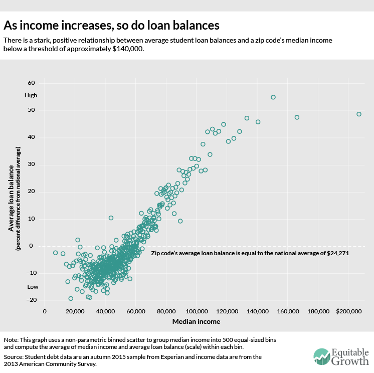
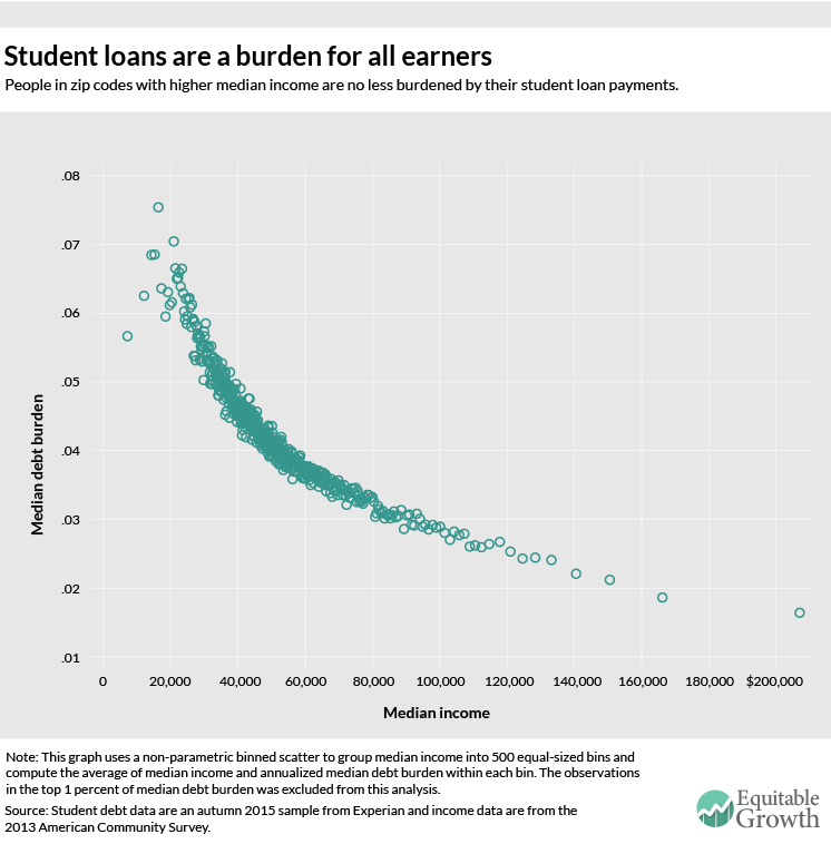
Figure 4 shows the relationship between the “burden” of student loan payments and zip code median income. Using the “average monthly payments on student loans” variable, we calculate that student debt absorbs around 7 percent of gross income in zip codes where median income is $20,000, declining to 2 percent in the highest-income zip code

Figure 4

These graphs show us that the burden of student debt isn’t just shouldered by the young. As borrowers age, servicing their student debt hinders their ability to accumulate wealth. In fact, the Pew Research Center found that college-educated householders with student debt have one-seventh the wealth of people without debt, in part because the wealthiest students don’t need to go into debt to pay for college. Student debt repayment may also delay expenditures that are associated with the traditional economic lifecycle, such as owning a home or a car or even getting married. Altogether, this new expense associated with attaining a middle-class income contributes to the erosion of middle-class wealth across generations.

As cumulative student debt continues to grow and we learn more about its role in the nation’s many economic problems, it is clear that a reconsideration of the policies that treat student debt as “good debt” because it finances valuable human capital is in order, especially in light of the problems that even young college graduates have in the labor market.

Methodology

This geographic analysis uses two primary datasets: credit reporting data on student debt from Experian and income data from the American Community Survey.

The Experian data includes eight key student debt variables (see Figure 5) aggregated from household-level microdata to the zip code level. The underlying household data are a snapshot of the entire U.S. population at a single point in time—in this case, the autumn of 2015.

Figure 5

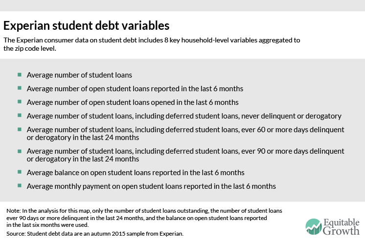
There are a number of caveats regarding the Experian data file that have guided our methodology for constructing variables and analyzing results:

• The universe of households contains only those with “any type of credit” and which, therefore, have a credit report. Relative to the population as a whole, this likely excludes the poorest households without any official credit access whatsoever.

• It is unclear how Experian constructs “households” since credit reports pertain to an individual’s credit history.

• If the same student loan has more than one signatory, then the loan may be assigned to multiple households and hence to multiple zip codes or even counted more than once within the same household.

• Experian claims that the universe of their geographically-aggregated data is all households with credit, but the levels of the data on loan balance and delinquency are more consistent with the idea that the universe is only households that have student loans. In other words, Experian claims their data include households that have credit but no outstanding student loans, but if that is the case the reported levels for both average loan balance and average delinquency are much higher than other sources would suggest. Average loan balance and average delinquency rates, however, are comparable to reliable outside estimates if interpreted as loan balance and delinquency among only those households with student debt.

For these reasons, we do not report any student loan data in dollar amounts. Instead, we have used two of the Experian variables to construct analogs to relative average household loan balance and relative delinquency.

To create the average household loan balance variable in the interactive map, we calculate an “average of the average” zip code-level student loan balance for the entire country, then code zip codes by percentage above or below that average-of-averages. For delinquency, we calculate a “delinquency rate” for each zip code by dividing the average number of 90-or-more-days-delinquent loans per household by the average number of outstanding loans per household. Then, after winsorizing the top one percent of observations to the 99th percentile value, we project the “delinquency rate” onto a scale that ranges from 0 to 10.

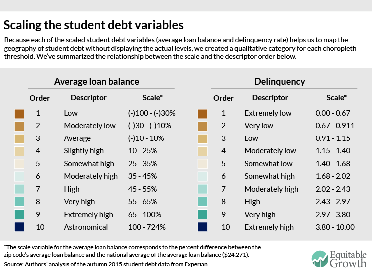
For user-friendliness, we assign each of these student debt scale variables a qualitative category. If average loan balance on the map is “somewhat high,” for example, then it means that a zip code’s average loan balance is between 25 and 35 percent higher than the national average of $24,271. Similarly, if the delinquency reads “very low,” it corresponds to a scale level between 0.067 and 0.091. Figure 6 summarizes the relationship between each of the scale variables’ levels and their qualitative description.

Figure 6

Next, we merge zip code-level median income data from the 2013 American Community Survey with our imputed scaled student debt variables in order to construct choropleth maps.

The actual map uses three different techniques to display the variables on a choropleth scale. For the average loan balance, we artificially set ten cutpoints to enhance the geographic variation in metropolitan areas; to do this, we maximized the breadth of the color categories for values higher than the average-of-averages loan balance. For delinquency, we created ten quantiles (or equal counts) to account for the right-skewed data. Finally, for median income, we used ten jenks (or natural breaks in the data) to assign the color scale. Higher numbers and darker shading correspond to higher household average student loan balances, higher shares of outstanding loans that are 90 or more days delinquent in the previous 24 months, and higher median incomes. We think that the geographic variation in the Experian data (and as seen in the maps) is believable, but not the levels reported by Experian.

Download the “Mapping Student Debt” presentation from the December 1, 2015 release (pdf)

*Correction, December 8, 2015: A previous version of this column cited a Department of Education projected graduate student default rate of 7 percent, but the Department has removed that projection from its website and we now think the 2 percent to 3 percent realized default rate is a better estimate.

Explaining the “History of Technology” series and equitable growth


Let me recite what history teaches,” wrote the 20th century American novelist Gertrude Stein. “History teaches.

Does history teach? In particular, does history teach about job destruction and creation? Can the study of history, both in case studies and in the broad strokes of trends, help us understand how structural changes in the U.S. economy have affected growth and inequality in the past? Can they give clues about what we can expect in the future?

The Washington Center for Equitable Growth set out to answer those questions by establishing a Working Group on the History of Technology. In a Washington, D.C. policy environment dominated by economists and political scientists, we wanted to see if the tools and concepts of the history of technology can be deployed in ways that complement those other disciplines. After all, historical precedents are routinely cited in policy discussions, but rarely are they subjected to the close analysis that professional historians can bring to the conversation.

Our working group of technology historians seeks to answer the question of whether there are elements of previous mass technological shifts that may aid in the management of workforce disruptions brought about by the post-high-tech revolution. The group considered this question in light of the overarching mission of Equitable Growth to investigate whether and how economic inequality affects economic growth and stability. By casting an informed look back to previous technology-driven job upheavals, we may find shifts in inequality and growth—shifts that indicate whether these phenomena are linked. If so, then perhaps answers to today’s growing income and wealth gaps will lie in some combination of spontaneous forces and active interventions by government or through public-private alliances.


The “History of Technology” series of essays

Equitable growth and Southern California’s aerospace industry
By Matthew H. Hersch, Assistant Professor of the History of Science at Harvard University
and a Research Associate of the Smithsonian Institution’s National Air and Space Museum

Not all inequality is the same: Slavery versus economic creativity in Civil War America
By John Majewski, Interim Dean of Humanities and Fine Arts and Professor in the Department
of History at the University of California, Santa Barbara

Engineering, industrialism, and socioeconomic orders in the Second Industrial Revolution: What U.S. policymakers today could learn from emerging technology professions and innovation at the turn of the 20th century
By Adelheid Voskuhl, Associate Professor of the History and Sociology of Science at the
University of Pennsylvania

Responsible innovation: The 1970s, today, and the implications for equitable growth
By Cyrus C.M. Mody, Professor and Chair in the History of Science, Technology, and Innovation
in the Faculty of Arts and Social Sciences at Maastricht University in the Netherlands

Energy transitions in the United States and
worker opportunities past, present, and future

By Christopher F. Jones, Assistant Professor in the School of Historical, Philosophical,
and Religious Studies at Arizona State University

Environmental regulation and technological development
in the U.S. auto industry

By Ann Johnson, Associate Professor, Department of Science and
Technology Studies, Cornell University

Emerging technologies, education, and the income gap
By Michael E. Gorman, Professor, Department of Engineering and Society, University of Virginia


We did not look for technological speculation or “futurism” in our work. But any technology that is or has been in operation for the last couple of hundred years has been fair game for our group, from the steam engine and railroad to nanoengineering, synthetic biology and microchip production, as well as the workforces related to those endeavors. Otherwise, in charging our group of historians, we brought no preconceptions in this regard. Nor do we think that there will necessarily be a clear line from previous experience to the future. Some past events and concepts might be a dead end, but some might provide a foothold, however modest, on understanding what lies ahead.

Whatever the case, historical lessons are too important to be ignored in considering the future of job creation in a post-high-tech world. In the words of the 18th century Scottish philosopher David Hume—a decidedly less musical but no less nuanced writer than Gertrude Stein—the future tends to resemble the past. The challenge, we might add, is ascertaining which tendencies will turn out to matter in the years ahead.

Jonathan D. Moreno is the David and Lyn Silfen University Professor at the University of Pennsylvania, where he teaches and researches medical ethics and health policy, the history and sociology of science, and philosophy. Moreno has served as an advisor to many U.S. governmental and nongovernmental organizations, including the Department of Defense, the Department of Homeland Security, the Department of Health and Human Services, the Centers for Disease Control and Prevention, the Federal Bureau of Investigation, the Howard Hughes Medical Institute, and the Bill and Melinda Gates Foundation. Moreno is an elected member of the National Academy of Medicine (formerly the Institute of Medicine) of the National Academies and is the U.S. member of the UNESCO International Bioethics Committee. 


What happened to the job ladder in the 21st century?

The job ladder, Veer.com

A few weeks ago, we published an analysis showing that the lowest-paying industries saw the largest increases in workers with a college degree between 2000 and 2014. Today, we follow that up by showing that the pattern is similar among young workers ages 19 to 34 (as opposed to workers with a college degree), but with one big difference—the oil, gas, and mining resource extraction and refining industries, which pay relatively well, saw a substantial increase in the share of young workers hired.

Considered alongside our previous results, this new analysis implies that resource extraction and refining industries provided an outlet for young workers without college degrees to attain well-paying employment. These industries profited from the development of hydraulic fracturing and other new technologies, as well as a worldwide boom in demand for natural resources that seems to have reversed since late 2014.

Figure 1

But these young adults working in the high-paid extraction and refining sectors obscures the larger picture of the U.S. job ladder: Outside those industries, young workers are increasingly being hired into low-paying ones. That is important to document because, as we discussed in our previous column, the education level for most workers in the U.S. Census Bureau’s Quarterly Workforce Indicators database is imputed rather than observed directly—and that imputation is potentially faulty since it is based on the 2000 Census. In contrast, the age of workers is observed directly for the vast majority of workers.

Figure 2

Looking at the share of young workers hired in each quarter between 2000 and 2014 yields further insight, which our colleague Kavya Vaghul discussed in part in her column last week on the impact of student debt on economic security. It divides industries into thirds based on their average earnings in 2000, then traces the share of hires in each industry that went to young workers. The share of young workers hired in high-paying industries shrank right at the onset of the Great Recession, while in its aftermath that share grew in low-paying ones. (See Figure 3.)

Figure 3

These findings are consistent with previous findings on the evolution of the job ladder during and after the Great Recession of 2007-2009, though our analysis indicates that the job ladder had already started deteriorating even before that, following the recession of the early 2000s.

The labor market has always been characterized by what economists call a “last in/first out” or “last hired/first fired” structure, meaning that workers who are laid off during recessions are generally those with the shortest job tenure, many of whom tend to be young. We also know that high-paying firms exhibited the greatest decline in hiring during the Great Recession. In combination, these two patterns imply that young adult workers disproportionately lost out at high-paying firms and industries, which is what the darkest green line in Figure 3 shows.

Following the Great Recession, employment grew most in low-wage jobs, so that is where young adults entering the workforce could find work—even if they had a college education. And because the high-wage firms and industries aren’t hiring, many of these workers are stuck in low-wage jobs. That failure of the job ladder portends dire consequences for young workers’ lifetime earnings since the peak years for job-switching and wage growth are the early ones. If these workers do not find opportunities to climb, then they will potentially be stuck on the lower income rungs for the rest of their lives.

Appendix

The construction of the U.S. Census Bureau’s Quarterly Workforce Indicators, the data from which these charts are constructed, is discussed in the appendix to our previous column. To make these charts on young adult workers’ share of hires, we define “young adult workers” as QWI age groups 2, 3, and 4 (comprised of workers ages 19 to 34), and we exclude groups 1 (ages 14 to 18) and 8 (ages 65 to 99) from the analysis entirely. Industry average earnings of full-quarter hires in 2000, or EarnHiraS, are deflated to 2014 dollars using the U.S. Consumer Price Index for all Urban Consumer, or CPI-U. When industries are divided into thirds according to earnings levels in Figure 3, the three groups are weighted by employment so that each group corresponds to approximately one third of the total U.S. workforce.

The observations excluded between Figures 1 and 2 are the North American Industrial Classification System (three-digit) industries 211 (Oil and Gas Extraction), 212 (Mining except Oil and Gas), 213 (Support Activities for Mining), and 324 (Petroleum and Coal Products Manufacturing, including Oil Refineries).

The pernicious effects of growing student debt on the economic security of young workers

Student debt illustration by David Evans, Equitable Growth

Student loans in the United States are now the second-largest source of debt, totaling $1.1 trillion shared among 42 million people with no sign of slowing down. Unfortunately, many questions about student debt, the characteristics of borrowers, and the nature of delinquency remain unanswered, primarily because agencies and researchers alike lacked access to the rich data in the U.S. Department of Education’s loan portfolio.

That changed last week when Adam Looney of the U.S. Department of the Treasury and Constantine Yannelis of Stanford University released an impressive new report that makes use of administrative data on student borrowing and earnings from linked, de-identified tax records to explore the student debt terrain.

Student debt nearly quadrupled over the past 15 years, and Looney and Yannelis find that the accelerated growth is largely due to a new type of borrower: students attending for-profit colleges. During the Great Recession, the number of students attending for-profit universities grew significantly in response to poor employment opportunities and a weak labor market. As a consequence, the number of borrowers grew too. Looney and Yannelis find that most of these “non-traditional” borrowers are vulnerable individuals who mostly come from lower-income backgrounds. Although average loan balances for borrowers who graduate from for-profit schools are smaller than those of nonprofit undergraduates or graduate students, these for-profit students face worse labor market opportunities, lower earnings, and, ultimately, much higher delinquency rates than their traditional college counterparts.

But just because the student loan crisis is concentrated among non-traditional borrowers does not mean that students attending a selective, non-profit, four-year university have it easy: The current labor market is not kind to young workers, even with traditional college degrees.

Young workers rely on job-to-job flows—transitioning between jobs to find better offers—in order to build their careers, move up the job ladder, and grow their earnings. Low unemployment allows workers to quit their jobs to search for more fruitful employment. When the labor market contracted during the Great Recession of 2007-2009, however, these job-to-job flows fell. Economists Giuseppe Moscarini of Yale University and Fabien Postel-Vinay of University College London find that during the recession, the jobs ladder shut down, trapping young workers in low-wage jobs. (See Figure 1.)

Figure 1

The danger for recent college graduates is that carrying a large load of student debt requires young people to remain employed, even at jobs that don’t pay well, and hence restricts their ability to search out better opportunities for long-term earnings growth.

Joseph Altonji, Lisa Kahn, and Jamin Speer of Yale University report that all recessions have a damaging long-term effect on recent college graduates no matter what they majored in. For the average major, a recession means a 10 percent reduction in earnings in their first year out of college. In past recessions, high-paying majors such as engineering were less adversely affected, but in the Great Recession, even an engineering degree wasn’t sufficient protection. The three researchers find that between 2007 and 2009, the effect of unemployment on earnings halved the relative advantage that a high-paying major previously guaranteed.

So if young, traditional college graduates are being challenged by the post-recession labor market, what happens when high levels of student debt are thrown into the mix? In a recent paper, Emmanuel Saez and Gabriel Zucman of the University of California-Berkeley find that between 1986 and 2012, the wealth of the bottom 90 percent of the wealth distribution in the United States didn’t grow at all. With the little wealth that is, it’s unlikely that recent graduates with large student debt are able to accumulate any savings after servicing their student debts. In fact, the Pew Research Center’s tabulations of the Survey of Consumer Finances show that college-educated householders under 40 who have student debt have one-seventh of the wealth of people who don’t.

Student debt is a long-term burden in other ways too. Paying off college loans displaces other costs associated with our traditional perception of U.S. adulthood and the economic life-cycle. Economists David Cooper and J. Christina Wang of the Federal Reserve Bank of Boston find that homeownership rates among college graduates ages 30 to 40 are lower for households with student debt. Similarly, other studies show that car ownership and marriage rates are also lower for young student borrowers.

As the student debt load grows for young borrowers, it is clear there may be long-term effects on young workers’ economic security. Just a generation ago, higher education was considerably more affordable or at least heavily subsidized by state governments, enabling young workers to begin saving and eventually realize the American Dream. But now, higher education is a transformative economic burden for the young workforce. And for the amount of student debt that graduates face upon entering the workforce, higher education certainly has not yielded commensurate benefits.

Putting the new U.S. Census data on income and poverty in context

Earlier this morning, the U.S. Census Bureau released new data on the state of incomes in 2014. According to the new data, the share of income going to the top 5 percent of American households is at 21.9 percent, a 0.3 percentage point decrease from 2013. Similarly, the Gini coefficient (a broad measure of income inequality) was essentially unchanged at 0.480. The official poverty rate stood still at 14.8 percent.

The important new data released today, however, are far from the only source of data on income and poverty trends in the United States. Other datasets paint a different story of family economic wellbeing. For instance, the flat levels of income inequality over the course of 2014 in the Census data diverge from evidence of rising inequality in other data on family incomes. Using tax data, University of California-Berkeley economist Emmanuel Saez finds that the share of income going to the top one percent increased by 1.1 percentage points in 2014. Understanding the state of income inequality and poverty in the United States means we have to be aware of what the Census data can and cannot tell us about the broader trends.

Case in point: it’s important to keep in mind what the Census Bureau considers as “income,” which can be defined in a number of ways. It could focus on income that’s earned strictly from work or investments (“market income”), or it could focus on income after accounting for the effects of government spending programs and taxes (“after-tax-and-transfer income”). The Census takes a third route with its preferred measure, called “money income.”

Money income includes some government programs (such as Social Security or unemployment compensation) but not all of them (such as in-kind transfers including the Supplemental Nutrition Assistance Program, also known as food stamps). It doesn’t include the value of some market income (such as employer-provided health insurance). And it doesn’t include the effects of taxation.

The difference between the Census’s definition of money income and data sources that use a different definition can paint different pictures of what’s happening to the U.S. economy.

Consider trends in income for the median household (the household that’s directly in the middle of the distribution of income in the United States). According to the Census Bureau data using money income, median household income dropped by 8.7 percent from 2000 to 2011. But Congressional Budget Office data on after-tax-and-transfer income shows a much different picture. Over the same time period, that data set shows median household income increasing by 13 percent. The CBO data on market income show a decline of only 4.3 percent. (See Figure 1.)

Figure 1

Something similar happens when we look at the poverty rate in the United States. The Census Bureau’s official poverty rate shows an essentially flat trend over the past few decades, rising only from 14 percent in 1967 to 15 percent in 2012. But the official rate doesn’t include the effects of many anti-poverty programs that aren’t straight cash transfers.

Researchers at Columbia University created a series that accounts for these additional programs among other factors, and the trend is quite different from the official series—poverty starts much higher at 26 percent in 1967 and then declines to 16 percent in 2012. So while this trend shows a decline in the poverty rate over the years (due mainly to an expanded social safety net), it also illustrates the significant share of the population still in poverty. In 2014, the supplemental poverty measure was slightly above the official poverty rate.

The Census has its own preliminary alternative measure of poverty (the “Supplemental Poverty Measure”) that takes into account the research communities’ findings on how best to measure poverty. Like the Columbia University team’s measure, the Supplemental Poverty Measure also includes many anti-poverty programs that offer “in-kind” support rather than cash benefits. Today’s Census data using the Supplemental Poverty Measure pegs poverty at 15.3 in 2014.

The data released today are an important update on the state of income and poverty in the United States. The Census data fill out a picture of a U.S. economy where too many families are struggling, and where the typical family’s income remains 6.5 percent lower than it was prior to the Great Recession. While the Census figures certainly aren’t the final word on the issue, this release is a key addition to our ability to understand some of the most important trends—inequality and poverty—in the U.S. economy today.