The employment effects of a much higher U.S. federal minimum wage: Lessons from other rich countries

Overview

Not long ago, most U.S. economists agreed that a statutory minimum wage with any “bite”—any meaningful effect on wages at the bottom of the labor market—would cause job losses and lead to a reduction in aggregate employment opportunities for low-wage workers. But as a result of path-breaking research by leading economists (first David Card at the University of California-Berkeley and Alan Krueger at Princeton University, and then by Arindrajit Dube at the University of Massachusetts-Amherst and Michael Reich at University of California-Berkeley and their associates, that has changed. Today, a vast majority of economists now understand that modest increases in the (currently very low) federal minimum wage would have little or no effect on overall job opportunities for minimum wage workers.

Download File
The employment effects of a much higher U.S. federal minimum wage: Lessons from other rich countries

Read the PDF in your browser

But what about the effects of a sizable increase of, say, more than double the current federal $7.25-an-hour minimum wage? What would a wage floor of $15 an hour mean for low-wage workers and U.S. economic growth?

This policy brief documents big differences in the national statutory minimum wage floor across several other affluent countries compared to the United States. The analysis shows how these differences translate into very large consequences for the incidence of low pay and the buying power of low-wage workers—using a wide variety of data, including workers’ starting pay and the famous “Big Mac” index of burger prices at McDonald’s restaurants in these countries—and concludes by reporting evidence that these substantial differences in approaches to low pay across the rich world show no correspondence to standard indicators of employment performance.

In short: Neither employment nor unemployment rates reflect the vast gap between the United States and other rich countries that have all but outlawed the payment of extremely low wages by establishing legal wage floors far above the U.S. federal minimum wage.

The minimum wage landscape in affluent nations

Rich countries have taken dramatically different paths on setting a lower boundary for wages. Some, including Denmark and the Scandinavian countries, have relied on extensions of collective bargaining agreements to set legal wage floors. This obviously is not how the U.S. labor market operates, so the focus of this issue brief is on those nations with statutory national minimum wages.

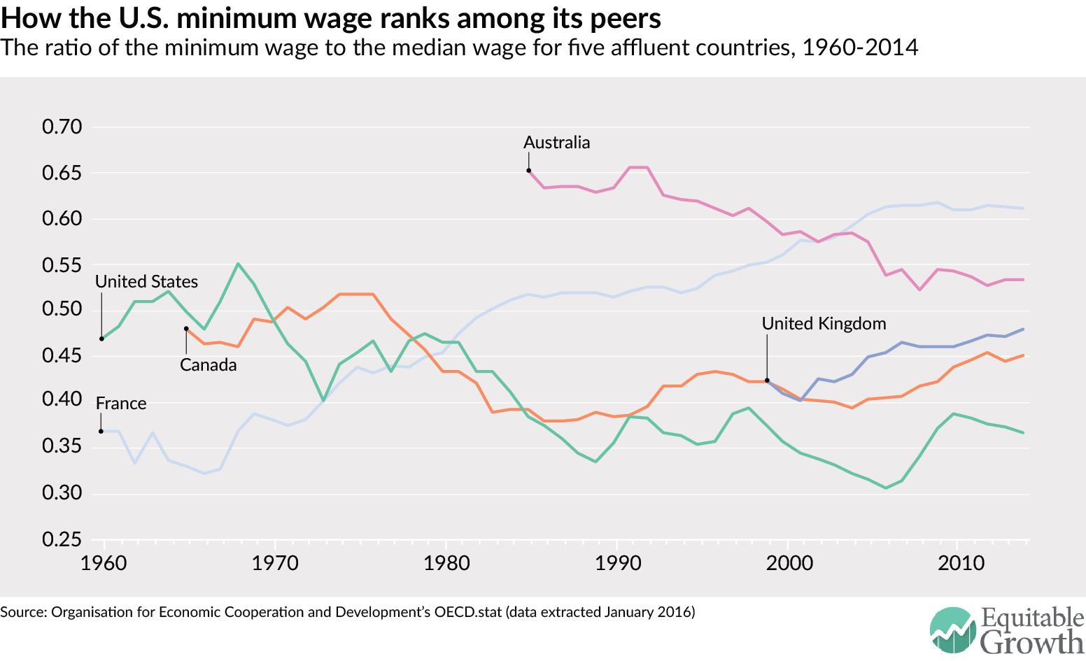
First, consider France. The French minimum wage climbed from about 35 percent of the median wage for full-time workers in the 1960s to 61 percent in 2014. In contrast, the U.S. minimum wage floor was around 50 percent of the median in the 1960s but has since fluctuated between 35 percent by the late 1980s and 37 percent in 2014. Then there is Australia, where the minimum wage also fell—from 65 percent in the early 1990s to 53 percent in 2014—but only because the country’s median wage rose faster than the statutory wage. Canada’s minimum-to-median wage rate followed about the same trajectory as the United States from the 1960s to about 1990 and has since ranged between 40 percent and 45 percent of the median wage, where it is today—well above the United States. The United Kingdom introduced a statutory minimum wage only in 1999, and as the chart shows, its value has increased relative to the median from about 40 percent in 2000 (like Canada) to 47 percent in 2014 (slightly above Canada and far above the United States). (See Figure 1.)

Figure 1

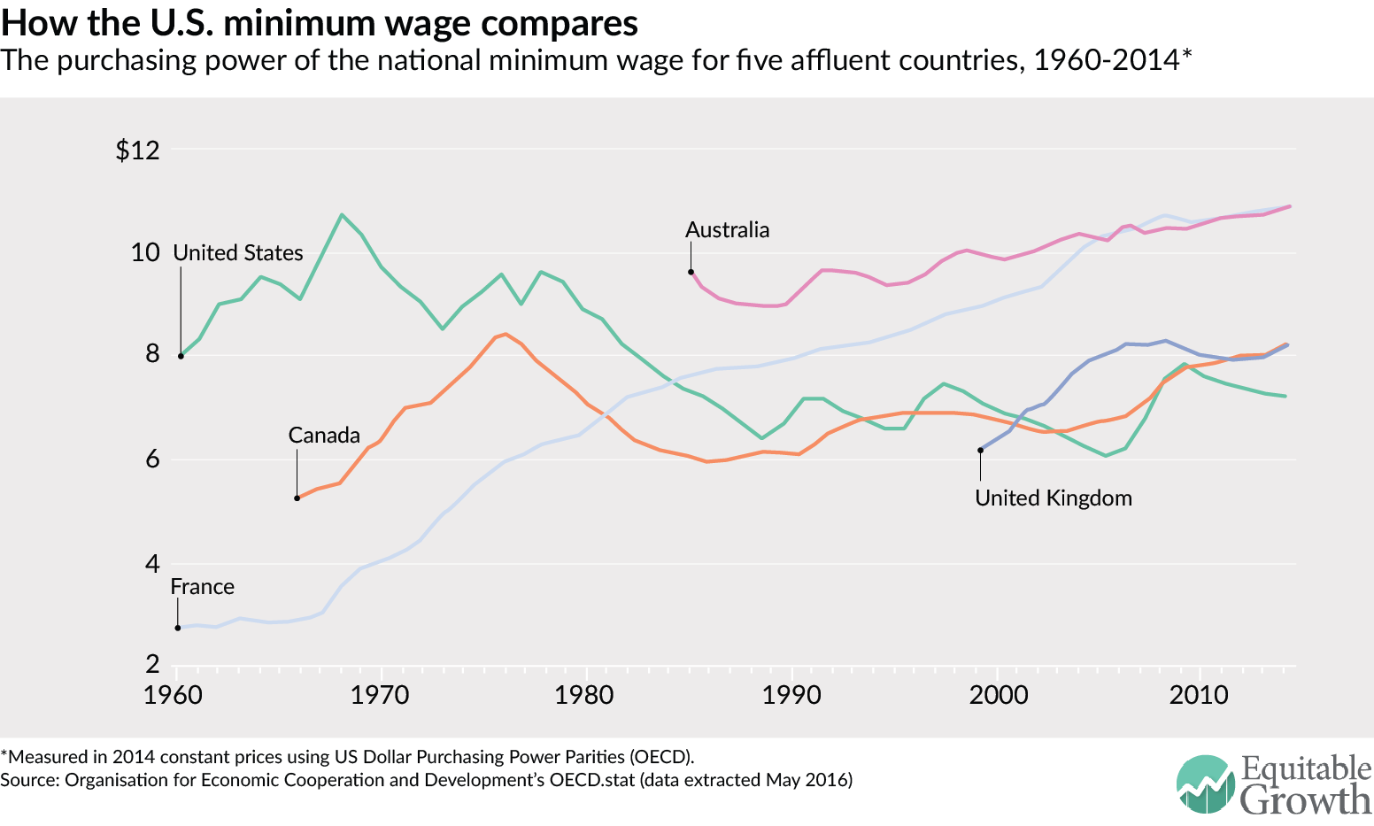
Another way to compare the minimum wage across national borders is in terms of purchasing power. The minimum wage in Australia and France buys a lot more than in the United Kingdom and Canada, and substantially more than in the United States. In Australia and France, the purchasing power of their minimum wage was equivalent to $10.90 in 2015. The wage floors in the United Kingdom and Canada are much lower—about $8.15 in 2015—but still considerably higher than the United States, where the federal minimum wage was $7.24 (below $7.25 because the figure uses 2014 constant dollars and there was slight inflation between 2014 and 2015). (See Figure 2.)

Figure 2

But the take-home pay of minimum-wage workers depends on both taxes and the effects on eligibility for benefits. A recent report on the minimum wage by the Organisation for Economic Cooperation and Development put it this way:

Without effective co-ordination, minimum wage hikes may not result in significant income gains for the targeted individuals, especially in countries where tax burdens on low-wage earners are sizeable, or where means-tested out-of-work transfers provide a comprehensive income safety net.

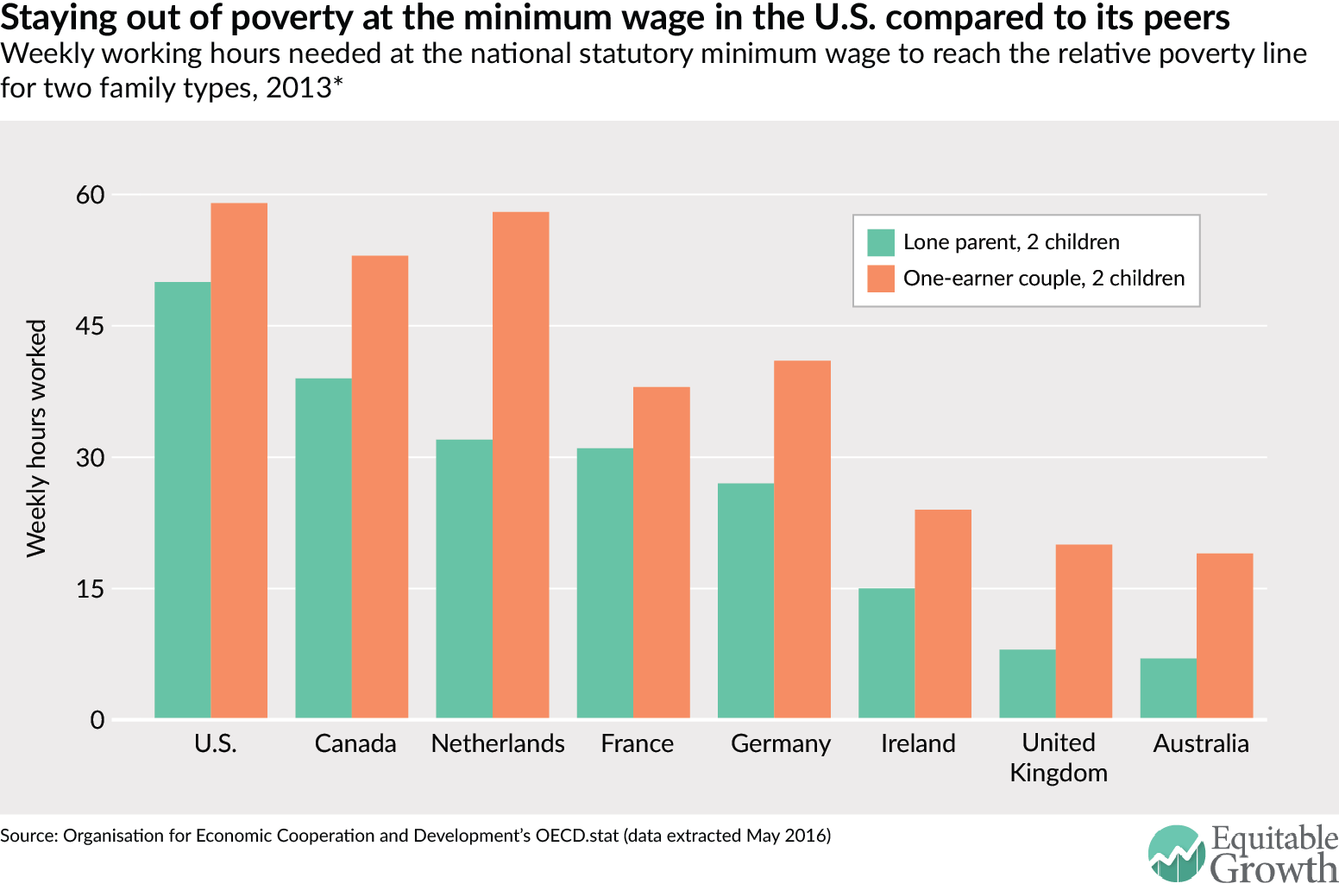
The OECD’s estimates of the weekly working hours a minimum wage worker needs to keep a family out of poverty varies enormously, from 50-to-59 hours in the United States (depending on the type of family) to 31-to-38 hours in France, to just 7-to-19 hours in Australia. Given taxes and benefits, Canada and the Netherlands are more like the United States, Ireland and the United Kingdom are more like Australia, and France and Germany fall in the middle. A one-earner couple with two children in the United States, for example, would require 59 hours of minimum wage work a week to keep that family out of poverty compared to 53 hours in Canada, 41 hours in Germany, 38 hours in France, 20 hours in the United Kingdom, and 19 hours in Australia. (See Figure 3.)

Figure 3

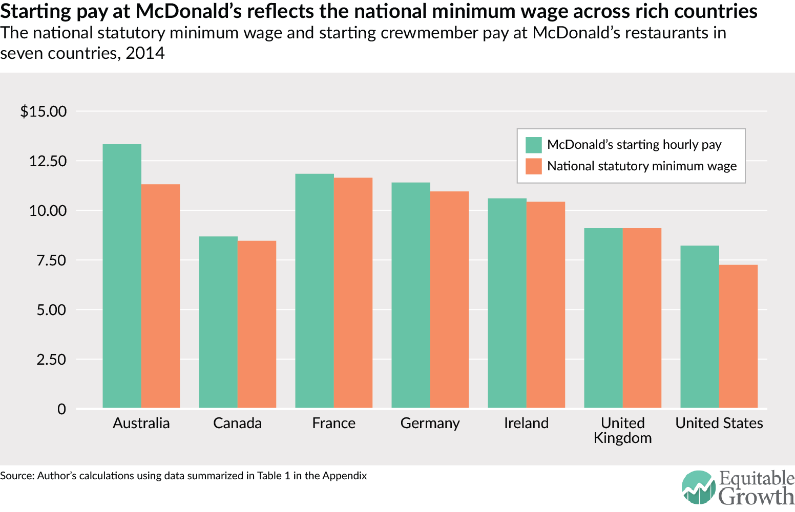
We can also get a good idea of the relative purchasing power of the minimum wage in different countries by comparing the starting wages at McDonald Restaurants, which is closely associated with the national minimum wage in each country, and by calculating the number of Big Mac burgers a minimum wage worker can buy for an hours work (at the pre-tax wage). The starting pay for a crewmember in these fast-food restaurants is, indeed, highly correlated with the nation’s minimum wage. In 2014, for example, starting pay at the restaurant chain in Australia averaged $13.33 compared to the minimum wage $11.31. This compared with $11.84 (and $11.64) in France, and just $8.22 (and $7.25) in the United States. The takeaway is that, not surprisingly, starting pay for fast food workers is far higher in countries that have a higher national minimum wage. (See Figure 4.)

Figure 4

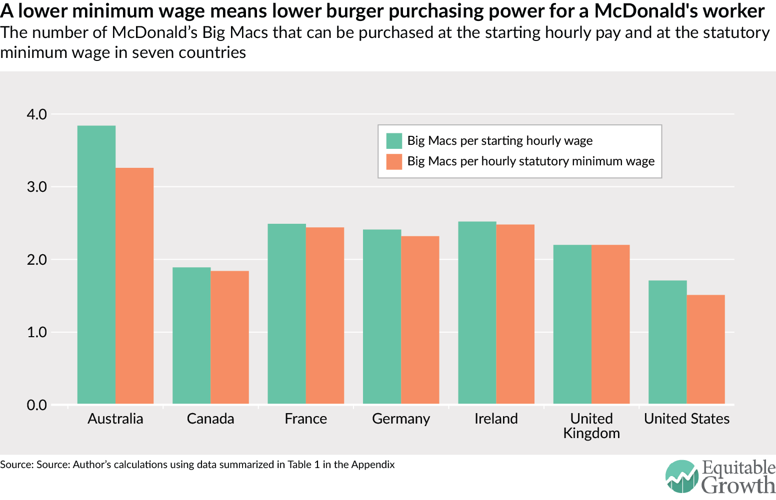
Not only is starting pay at McDonald’s extremely low in the United States compared to other rich countries, but so too is the price of a Big Mac relatively high in this country compared to other affluent countries. The combination of low pay and high prices means that the number of Big Macs a McDonald’s entry-level worker can buy is 3.8 in Australia, 2.5 in France and only 1.7 in the United States. The pattern is the same for workers’ ability to buy Big Macs at the national minimum wage: 3.3 in Australia, 2.4 in France, and 1.5 in the United States. (See Figure 5.)

Figure 5

The employment effects of the minimum wage in the United States and other affluent countries

According to conventional thinking, there are big wage-employment tradeoffs associated with a high minimum wage. As a result, while there may be some low-wage workers in Australia and France who will benefit from higher wages, many will be “priced-out” of a job. In this view, a higher minimum wage, together with higher rates of collective bargaining (among other factors) explains cross-country differences not only in the incidence of low pay, but in employment and unemployment rates for minimum wage workers.

If these so-called “labor market rigidities” price workers out of the labor market, then reducing the low-wage share of employment (via a higher minimum wage) should also reduce the low-education employment rate because young, less-educated workers should have a harder time finding and keeping jobs.

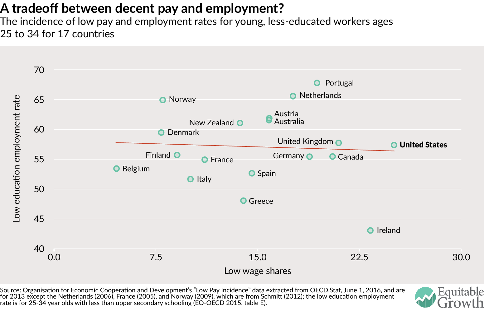
Yet the data offer little support for this orthodox tradeoff view. Rather, OECD data show that while there is a huge 14-percentage point gap in the low-wage share of employment between France (11 percent) and the United States (25 percent), the employment rates for young, less-educated workers are only moderately higher in the United States (57.4 percent compared to 54.9 percent). Similarly, Australia’s incidence of low pay is more than 10 percentage points below the U.S. level, but the low-education employment rate is more than 4 points higher, illustrating the lack of any statistical relationship across affluent countries between the incidence of low pay and the employment rate for less-educated young adults. (See Figure 6.)

Figure 6

But what about youth unemployment rates? There are two alternative unemployment rates that enable comparisons across countries. One is unemployment measured as a share of the labor force; the other is unemployment as a share of the working age population. Comparing these two measures in the United States and France and in the United States and Australia among young workers ages 15 to 24 shows no obvious correspondence between either measure and the level or trajectory of the national minimum wage.

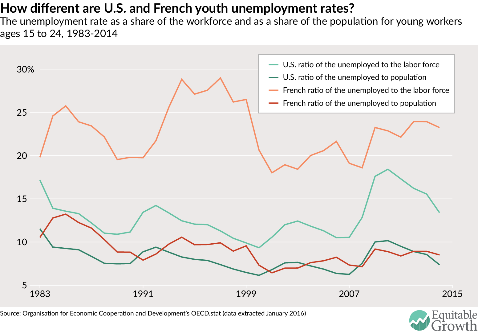
First let’s look at the United States and France. If the conventional wisdom were correct, then United States-French youth unemployment rates should have sharply diverged. But what we see instead is considerable convergence. From 1997 to 2007 the French unemployment rate for 15-to-24 year olds fell dramatically, from 30 percent to 19.1 percent, while the U.S. rate increased from 11.3 percent to 12.8 percent, and France continued to close the unemployment gap between 2007 and 2010 (see Figure 7). This 1997-2007 convergence took place as the French minimum wage increased from 54 percent to 62 percent of the nation’s full-time median wage while U.S. federal minimum wage fell from 39 to 31 percent—exactly half the French ratio (see figures 1 and 2). Over the entire 1997-to-2014 period, the conventional French unemployment rate improved by 6.8 percentage points and the U.S. rate worsened by 2.1 points.

Figure 7

Figure 7 also compares France and the United States on a much better measure of youth unemployment: the unemployment-to-population rate. This indicator shows that these countries have tracked each other closely since 1983, with the rate in both countries fluctuating between 6 and 10 percent. In short, neither unemployment measure shows any evidence of the predicted divergence in French-U.S. employment performance.

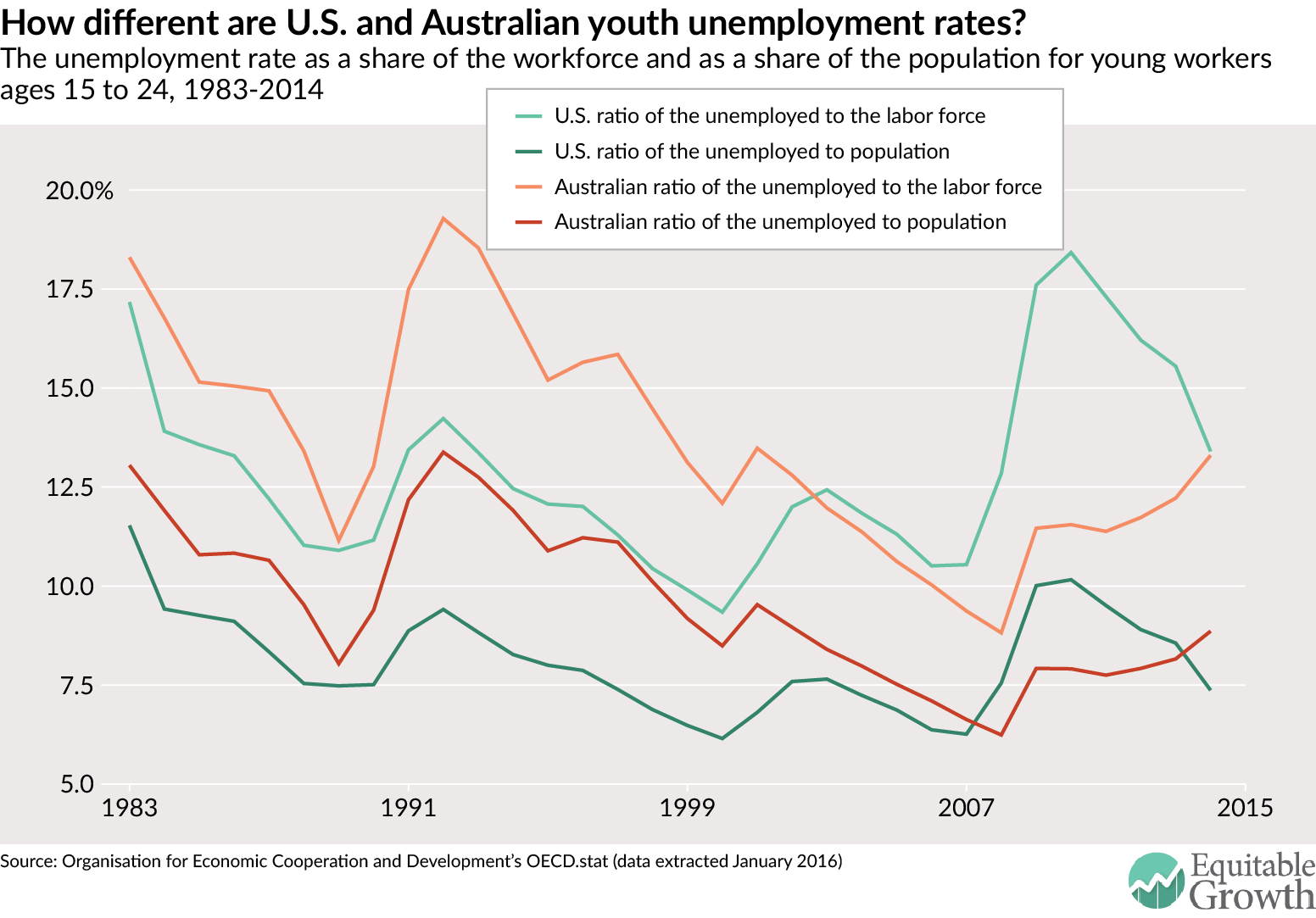
Comparing these two unemployment-rate measures for Australia and France also fails to confirm the conventional tradeoff prediction. As in France, Australia has legislated a high minimum wage by international standards. (See Figures 1 and 2.) Yet, by both indicators, youth unemployment fell sharply between the early 1990s and the global 2008-2010 economic crisis—to levels below the United States. (See Figure 8.)

Figure 8

Other affluent countries provide much higher and more universal support for working families than the United States, in the form of health care, housing, education, and child subsidies. This means the legal wage floor must carry a much higher burden for maintaining minimally decent incomes for working families than in other rich countries.

Yet, as the data presented in this policy brief demonstrates, the United States is at the extreme low-end among affluent countries on the level of the minimum wage, whether measured in terms of buying power or relative to the median wage. (See Figures 1 and 2.)
As a result, after taking into account taxes and benefits, it typically takes a minimum wage worker six to seven times as many hours of work per week to keep a lone parent or two child family out of poverty compared to the United Kingdom or Australia (50 hours versus 7 or 8 hours). (See Figure 3.)

This gigantic gap in the payoff to working at the minimum wage for U.S. workers can also be illustrated by the much lower starting pay at McDonald’s franchises, and the far fewer Big Macs a U.S. worker at McDonald’s can buy with an hour’s work than her counterparts in other rich countries. (See Figures 4 and 5.) At the same time, standard measures fail to show the predicted worsening of youth employment performance between the United States and countries that set a much higher legal wage floor, such as Australia and France. (See Figures 6, 7, and 8.)

All of this international evidence strongly suggests that, properly designed and implemented, much higher living standards are possible for working families in the United States by setting the federal minimum wage far above the current level of $7.25 without affecting overall employment opportunities for minimum-wage workers.

—David Howell is a professor of economics and public policy at The New School in New York City. This note reflects and builds on the material that appears in the Washington Center for Equitable Growth working paper, “What’s the Right Minimum Wage? Reframing the Debate from ‘No Job Loss’ to a ‘Minimum Living Wage,” co-authored with Kea Fiedler and Stephanie Luce. Special thanks to Kea Fiedler for her work on the McDonald’s data.

Photo by Remy De La Mauviniere, Associated Press

The misplaced debate about job loss and a $15 minimum wage

Overview

The leading criticism of the “Fight for $15” campaign to raise the federal minimum wage to $15 an hour is the presumed loss of jobs. Employers, the argument goes, would eliminate some workers or reduce their hours in the short-term, and in the longer run, further automate their operations in order to ensure that they will need fewer low-wage workers in the future. For many leading minimum wage advocates, even a gradually phased-in $12 wage floor would take us into “uncharted waters” that would be “a risk not worth taking.”

On the other side is the long historical concern with making work “pay,” even if that means some job loss. In this view, the most important consideration is the overall employment impact on low-wage workers, after accounting for the additional job creation that will come with higher consumer spending from higher wages, which will almost certainly at least offset any direct initial job losses. And even more importantly, what really matters in this view are the likely huge overall net benefits of a large increase for minimum-wage workers and their families.

Download File
The misplaced debate about job loss

Read the PDF in your browser

If we are serious about job opportunities for low-wage workers then there are many effective ways to compensate those who lose their jobs, ranging from expansionary economic policy to increased public infrastructure spending, more generous unemployment benefits and above all, public-sector job creation. A related issue is whether it makes moral, economic and fiscal sense to maintain a low federal minimum wage and then ask taxpayers to subsidize the employers of low-wage workers by propping up the incomes of poor working families only via means-tested programs such as the Earned Income Tax Credit and supplemental nutrition assistance.

The debate has been, effectively, a stalemate, with the federal minimum wage set at extremely low levels ($7.25 since 2008) by both historical and international standards. Part of the explanation for our persistent failure to establish a minimally decent wage floor at the federal level has been the way the discourse has been framed—even by many of the strongest advocates for substantially higher minimum wage.

In recent years, the best evidence shows that moderate increases from very low wage floors have no discernible effects on employment, which has helped make the case for substantial increases in the minimum wage. But the very strength of this new evidence— research designs that effectively identify employment effects at the level of individual establishments—has contributed to the adoption of a narrow standard for setting the “right” legal wage floor—defined as the wage that previous research demonstrates will pose little or no risk of future job loss, anywhere. For all sides, the central question has become: Whose estimate of the wage threshold at which there is no job losses whatsoever is the most credible?

Some economists, for example, point to existing evidence that the effects on employment when the minimum wage is increased within the $6-to-$10 range are minimal. Yet other researchers continue to argue, with credible statistical support, that sizable increases within this $6-to-$10 range do cause at least some job loss in some establishments in some regions, even if limited to high-turnover teenagers.

But there certainly is no evidence that can be relied upon to identify the no-job-loss threshold for a legal wage floor that would apply to the entire United States—the wage below which it is known that there is little or no risk of job loss anywhere, and above which there is known to be a risk of job loss that is high enough to be not worth taking. The only truly reliable way to do this would be to regularly increase the federal minimum wage while carefully monitoring the employment effects, much as the United Kingdom’s Low Pay Commission has done for the minimum wage that was instituted there in 1999.

There are different stakeholders in this debate. On the one side, there are the academic economists who care deeply about empirical confirmation of price-quantity tradeoffs and restaurant owners who care equally as much about their profit margins. On the other side, there are workers and their advocates who desire the establishment of a minimum living wage. Given the many parties with a big stake in the outcome, relying on evidence-based criteria about job loss for setting the wage floor all but guarantees unresolvable controversy.

The methodological double bind in setting the minimum wage

Then there is the methodological problem—a classic case of “Catch 22.” Because the identification of the wage at which there is expected to be zero job loss must be evidence-based, there is no way to establish the higher nationwide wage floors necessary for empirical tests. There are other places that have enacted higher minimum wages—think Santa Monica, Seattle, New York state, France, Australia or the United Kingdom—but they would face the same problem if they relied exclusively on zero job loss as the criterion for the proper wage floor. In practice, high minimum wage locations have relied on other criteria when making the political choice to set the legal wage, namely a wage that more closely approximates a minimum living wage than what the unregulated market generates.

In practical terms, local and state government’s past reliance on statistical tests for other jurisdictions not only means that we must assume that they are directly applicable (why would evidence from Seattle, New York state or the United Kingdom be a reliable guide to the effects at the level of the entire U.S. labor market?), but also requires that places imposing a no-job-loss standard must always lag far behind the leaders, and effectively condemns them to setting the wage floor well below the actual wage that will start generating job loss. In short, the no-job-loss criterion cannot stand on its own as a coherent and meaningful standard for setting the legal wage floor, and by relying on old statistical results from other places, ensures a wage that is too low on it own terms.

Ignoring the net benefits of raising the minimum wage

When the criterion for raising the minimum wage is concerned only with the cost side of an increase, the costs of some predicted job losses are all that matters. If the wage floor is set above the no-job-loss level, what kind of jobs will be lost? Who will be the job losers? What alternatives were available to them? These are the kinds of questions that must be asked to determine the costs of minimum wage related job losses. But there are obviously benefits to raising the legal wage floor. Shouldn’t they be counted and compared to the costs?

Those benefits are evident directly for the workers receiving wage increases as a result of a rise in the minimum wage, either because they are earning between the old minimum wage and the new one (say, between $7.25 and $15) or because they earn a bit above the new minimum wage—because employers increase wages to maintain wage differentials among workers by skill or seniority. The benefits also are evident for taxpayers–with a much higher minimum wage there would be less need to rely on means-tested redistribution to increase the after-tax and benefit incomes of working families.

Forgetting the ethical and efficiency arguments for raising the minimum wage

Relaying on the no-job-losses criterion for setting an appropriate federal wage floor entirely ignores the main traditional justification for the minimum wage: The moral, social, economic, and political benefits of a much higher standard of living from work for tens of millions of workers. On both human rights and economic efficiency grounds, workers should be able to sustain at least themselves and ideally their families. And on the same grounds, it is preferable to do so from their own work rather than from either tax-based public spending or private charity.

It is hard to put this argument for a living wage better than Adam Smith did several centuries ago:

A man must always live by his work, and his wages must at least be sufficient to maintain him. They must even upon most occasions be somewhat more; otherwise it would be impossible for him to bring up a family…. No society can surely be flourishing and happy, of which the far greater part of the members are poor and miserable.

A public policy straightjacket

Determining a suitable federal minimum wage based solely on a zero job loss rule is a public policy straightjacket that would effectively rule out any significant raise of the wage floor above that which already exists. Yet from a historical perspective, strict adherence to such policymaking criteria would have also made it impossible to ban child labor (job losses!), as well as many critical environmental and occupational health and safety regulations. It would also foreclose any consideration of policies like paid family leave, which exists in every other affluent country.

Conclusion

Breaking out of this public policy straightjacket requires policymakers to rethink their criteria for raising the minimum wage. It also means that economists must shake off their fear of challenging the prevailing orthodoxy—a no-immediate-harm-to-anyone way of thinking—and see the longer-term benefits to millions of workers. It is estimated that the move to a $15 minimum wage by both California and New York state will directly raise the pay for over one-third of all workers.

If we really care about maximizing employment opportunities then we should not hold a decent minimum wage hostage to the no-job-loss standard. Rather, we should put a much higher priority on full-employment fiscal and monetary macroeconomic policy, minor variations of which would have massively greater employment effects than even the highest statutory wage floors that have been proposed.

But it is also well within our capabilities to counter any job loss that can be linked to the adoption of what the prominent University of Chicago economist J. B. Clark in 1913 called “emergency relief” such as extended unemployment benefits, education and training subsidies, and public jobs programs. A minimum living wage combined with other policies common throughout the affluent world, such as meaningful child-cash allowances, would put the United States back among other rich nations that promote work incentives while all but eliminating both in-work poverty and child poverty. It would put the country into waters that most other affluent nations have charted and are already navigating.

—David Howell is a professor of economics and public policy at The New School in New York City. This note reflects and builds on the material that appears in the working paper published by the Washington Center for Equitable Growth, “What’s the Right Minimum Wage? Reframing the Debate from ‘No Job Loss’ to a ‘Minimum Living Wage,’” co-authored with Kea Fiedler and Stephanie Luce.

Photo Uncredited, Associated Press

Working mothers with infants and toddlers and the importance of family economic security

Anne Quirk and her 11-month-old son Kieran play in the front yard of their home in Providence, R.I.

Overview

For families in the United States with children ages five and under—whether in married- or single-parent homes—mothers have been essential to bolstering economic security. Mothers’ increased working hours helped stabilize and boost family income. In the face of decreasing economic security, though, these large increases in hours worked by mothers, especially in households with young children who require physical and emotional care and nurturing, comes at a price: time.

As more mothers spend their days outside of the home trying to deliver much-needed financial stability, we need to understand the consequences of their work. As Heather Boushey documents in her book, “Finding Time: The Economics of Work-Life Conflict,” families now rely on those added hours and earnings of women. But for different types of families the transformations in the women’s role at home and at work mean different things. Especially for families with an infant or pre-school aged child, the challenges of how to address work-life conflicts can be acute. Without sufficient social infrastructure to help while parents are at work —such as paid family leave, paid sick days, flextime, predictable schedules, childcare, or universal high-quality prekindergarten programs—families are increasingly struggling to balance economic security with caregiving at home.

Download File
Working mothers with young children and family economic security (pdf)

Read the full pdf in your browser

This issue brief builds on the findings from “Finding Time” and explores how women’s increased hours of work and higher earnings have affected the incomes for families with young children. We unpack the role that women have played in helping stabilize family incomes across married-parents and single-parents with children age five or younger. Our findings are telling:

  • Across the board, married-parent families with young children have higher incomes than single-parent families, although between 1979 and 2013 both married- and single-parent families increased their incomes at similar low rates.
  • While in both 1979 and 2013 women from married-parent families worked more hours than single-mothers with young children, both groups of women saw similar and significant increases in their hours of work across all income groups.
  • The rise in women’s hours have been important for trends in family income. Between 1979 and 2013, in both married- and single-parent families, women’s earnings from higher wages and added hours have been positive across all income groups. In fact, for families with young children, women’s earnings from more working hours in particular was substantially large.

The changing role of women and the composition of families

Over the past four decades in United States, the composition of families with children has changed markedly. Most importantly, there is an increase in diversity of family types. There is no longer a dominant “typical” family, especially not one with a breadwinning father, a care-taking mother, and their dependent children. Instead, there is a wide array of family types. Our definition of who comprises a family now—more than ever before—has expanded to include singles living alone, biologically unrelated individuals, or even a boarder who joins in on family dinner and helps out with homework.

Trends in marriage and fertility have both contributed to greater family complexity. Marriage (if it happens at all) happens later in life, and the median age of first marriage is now 29 for men and 27 for women—higher than at any point since the 1950s. And, of course, same sex marriage is now legal across the nation. At the same time, many women are delaying childbearing and the typical woman has her first child now at age 26. Further, children are increasingly being born into families with unmarried parents; in 2014, 40.3 percent of all births in 2014 were to an unmarried mother. What this means is that there is more complexity of family types.

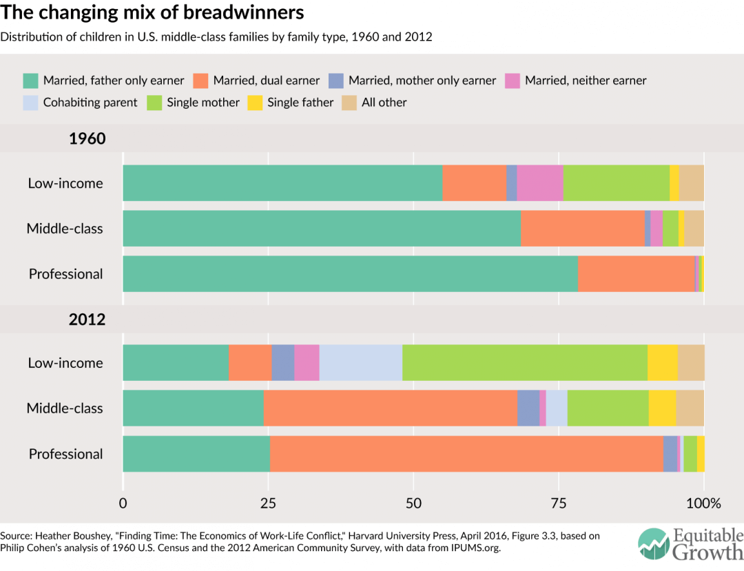
A second set of changes is who works and what this looks like across the income spectrum. While it used to be that most children were raised in married-couple families, be they at the top or the bottom of the income ladder. Now, however, while families at the top continue to raise children inside marriage—typically with both parents holding down a fairly high-paying job—children in families at the bottom of the income distribution—and now many in the middle—are living with a single, working parent, most often a mother. (See Figure 1.)

Figure 1


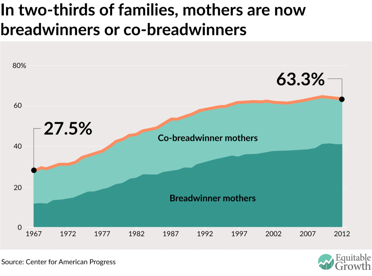
While families have become more complex, incomes have become more unequal. Faced with greater economic insecurity, families had to find ways to cope. One strategy was for women to increase their engagement with the economy. Initially, the “American wife” with school-age children migrated to the workforce, and soon after those with even younger children joined in. As women became more integrated into the workforce, they eventually became their families’ breadwinners, with two-thirds now either the main breadwinner or sharing that responsibility with their husband.

Using data from the Current Population Survey, we chronicle how family incomes changed between 1979 and 2013 for low-income, middle-class, and professional families by family type. Specifically, we decompose these changes over time into differences in male earnings, female earnings from higher wages, female earnings from more hours worked, and other sources of income, which include Social Security and pensions. (See Box.)

Defining income groups and family types

The analysis in this issue brief follows the same methodology presented in “Finding Time.” For ease of composition, we use the term “family” throughout the brief even though the analysis is done at the household level. We split households in our sample into three income groups:

  • Low-income households are those in the bottom third of the income distribution, earning less than $25,440 per year in 2015 dollars.
  • Professional households are those in the top fifth of the income distribution who have at least one household member with a college degree or higher; these households have an income of $71,158 or higher in 2015 dollars.
  • Everyone else falls in the middle-class category.

In this issue brief, we also refer to two different family types who have “young” (age five or less) children:

  • Married-parent families: The parents are married and at least one own young child is present in the household. (Unfortunately, at this time, the data limit our analysis heterosexual couples only.) Within these households, other, older children or adults, related or not and including adult-age children may be present and may contribute to the family’s income. Most families in this category, however, have two parents and their children alone.
  • Single-parent families: Either the mother alone or the father alone and at least one young child is present within the household. Within the household, there are no other adults related or unrelated adults who have earnings from a job or income from other sources.

Our sample only includes working-age families, where at least one person in the household is between the ages of 16 and 64.

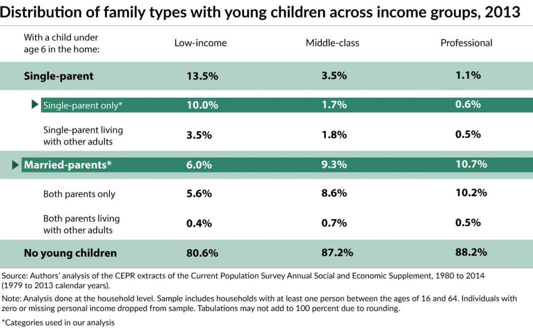
In the United States, only 19.1 percent of families have a child under age six. Table 1 shows the distribution of married parent and single-parent families across the income spectrum with and without one or more young children at home. Due to small sample sizes for certain groups, we were unable to conduct our analysis for a variety of family types, but we can break down the shares of different types of families by income group. For the purposes of this analysis, we select households where both parents are married from the “both parents only” and “both parents living with other adults” categories to get our “married-parent” families. For our “single-parent” families, we select households from the “single-parent” category. These are bolded in Table 1.

Table 1


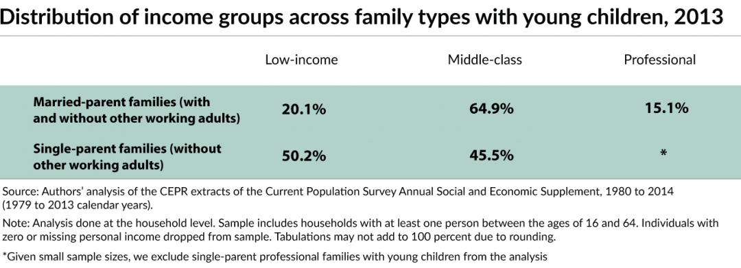
Table 2 breaks down the sample for this analysis, showing the share of each of these family types across the three income groups for 2013. Notably, the share of single-parent families decrease as we move up the income ladder. We exclude single-parent families with young children from our analysis of professional families as the sample size is too small.

Table 2


Setting some context

Before turning to the decomposition analysis, let’s first set some broad context for how family incomes and women’s hours changed between 1979 and 2013 for low-income, middle-class, and professional families with young children.

How did income change between 1979 and 2013 for families with young children?

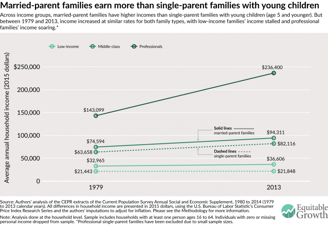
Between 1979 and 2013, while married-parent families had higher family income than single-parent families with young children, both types of families saw similar rates of growth in their income. (See Figure 2.)

Figure 2


Low-income families

Figure 2 shows that between 1979 and 2013, low-income families with young children—both married and unmarried—saw a slight rise in their incomes. Married-parent families with young children earned substantially more than single-parent families. In 1979, low-income married-parent homes, on average, brought in $32,965 annually compared to the $22,443 earned by single-parent families with children age five and under. By 2013, these disparities still persisted, with married-parent families earning $36,606 and single-parent families earning $21,848 annually.

The gap in average annual income between married-parent and single-parent family types can be often—but not always—explained by simple addition: Married-couples, now more than ever before, often have two sources of income. Although low-income single-parent families had a smaller annual income, on average, than married-parent families, between 1979 and 2013, both their incomes grew at relatively small rates (1.9 percent and 11.0 percent, respectively). These rates of income growth for families with young children indicate that income stalled.

Middle-class families

Figure 2 also shows that for middle-class families with young children, income rose between 1979 and 2013. As was the case for families across the low-income group, middle-class married-parent families with young children earned more, on average, in 1979 and 2013 than single-parent families. Yet, despite earning more, married-parent families’ income had similar rates of growth to single-parent families’; between 1979 and 2013, both married- and single-parent families with children age five and under grew their incomes by 26.4 percent and 29.0 percent, respectively.

Professional families

Across the board, Figure 2 also shows that between 1979 and 2013, professional families with young children have seen their incomes soar, and married-families with young children, in particular, have seen outstanding gains. In 1979, professional married couple families with young children earned, on average, $143,099. By 2013, their average annual income had grown by 65.2 percent to $236,400. The gap between married-parent professional families’ income and low-income and middle-class families’ income has widened markedly over the past four decades.

How did women’s working hours change between 1979 and 2013 for families with young children?

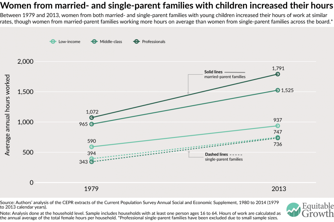
Taking a look at the hours that women from different families and income groups work gives us some insight into why families with young children increased their incomes between 1979 and 2013. Across the board, over the past four decades, women from married-parent and single-parent families grew their hours of work markedly. (See Figure 3.)

Figure 3


Low-income families

Figure 3 shows that in 1979, mothers of young children (and other working women) in married-couple families worked 590 hours annually (about 11.4 hours per week) and single-mothers worked 394 hours (7.6 hours per week). By 2013, women from both low-income married- and single-parent families with young children had grown their annual hours of work by 67.0 percent and 89.8 percent to 937 hours (18.0 hours per week) and 747 hours (14.4 hours per week), respectively.

Middle-class families

Just like women from low-income families, Figure 3 shows that women from middle-class families with young children greatly increased their hours at work between 1979 and 2013. In 1979, women from middle-class married-parent and single-parent families with children age five and under worked an annual average of 965 hours (or 18.6 hours per week) and 343 hours (6.6 hours per week), respectively. In 2013, women from married-parent families with young children had increased their hours of work by 58.1 percent to 1,525 hours annually (29.3 hours weekly), and mothers in middle-class single-parent families had more than doubled their hours (an increase of 114.5 percent) to 736 (14.2 hours weekly).

Professional families

Again, like we noted for other income groups, for professional families, women from homes with children age five and under had large increases in their hours of employment. Figure 3 shows that among professional families in 1979, women in married-couple families worked an annual average of 1,072 hours (20.6 hours per week), growing their hours by 67.0 percent to 1,791 annually (34.4 hours weekly) by 2013.

Though mothers (and other women) in professional married-couple families work more hours than middle-class and low-income, the rates of increase are relatively comparable across the board, corroborating the narrative that more and more women with young children have joined the workforce.

Decomposing the changes in income for families with young children

In Figure 2, we saw that between 1979 and 2013, across the board, married-parent families have higher incomes but similar rates of increase in income to single-parent families with young children. Figure 3 highlights that women from families with young children have been working more hours and perhaps have seen some of the largest increases in their hours at work.

Given these broad trends, a natural question arises about how the large increases in women’s hours relate to the large increases in family income for these families with young children. To unpack this correlation, we decompose the changes in families’ average household income between 1979 and 2013 into male earnings, female earnings, and income from other non-employment-related sources, which include Social Security and pensions and other sources.

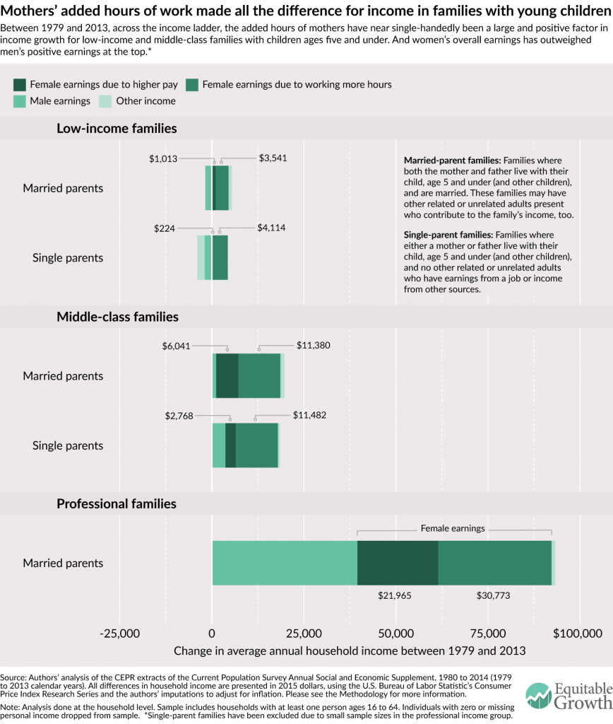
Specifically, we divide female earnings into two parts: the portion due to women working more hours per year and that due to women earning more per hour. To calculate female earnings stemming directly from the additional hours worked, we take the difference between the 2013 female earnings and the hypothetical earnings of women if they earned 2013 hourly wages but worked the same hours as women did in 1979. (For more on how we did this calculation, please see our Methodology.) We find that within families with young children across the income ladder, the added hours of mothers have near single-handedly been a large and positive factor for income growth for low-income and middle-class families while women’s earnings overall have outweighed men’s positive earnings at the top. (See Figure 4.)

Figure 4


Low-income families

Figure 4 shows that for low-income families with young children, both women’s earnings from more hours and from higher wages protected against falling family incomes between 1979 and 2013. For married- and single-parent families with children five and under, men’s earnings pulled income down at varying degrees. Men in married-parent families and fathers in single-parent families lost $1,748 and $1,938 in earnings between 1979 and 2013, respectively.

In contrast, women’s added hours and higher pay boosted incomes in both low-income family groups. For low-income married-parent families with young children, women’s higher wages increased family incomes by an average of $1,013 while women’s added hours grew family income by an average of $3,541. Single-parent families saw similar substantial gains in mother’s economic contributions: Between 1979 and 2013, women’s higher wages contributed $224 to earnings and added hours boosted incomes by $4,114.

The changes in “other income” are also of interest. For low-income married-parent families, other income grew by $860, but for single-parent families, other income decreased by $1,997. For single-parent families, this decrease in reliance on other sources of income—which could include federal transfers such as supplemental nutrition assistance and Temporary Assistance for Needy Families as well as Social Security benefits—indicates that these policies may not be adequately supportive or sensitive to the needs of parenting alone.

Middle-class families

Across the board, middle-class families, like low-income families, saw positive increases in their income largely due to the contributions of women and their increased labor force participation. Figure 4 shows that for both middle-class married- and single-parent families of young children, male earnings made a relatively small, positive addition of $1,205 and $3,706, respectively.

Women’s earnings, in contrast, were positive and large. Women’s earnings from higher wages added $6,041 and $2,768 for married-parent and single-parent families, respectively. The additions due to women’s added hours at work were more impressive, as women from married- and single-parent homed secured an additional $11,380 and $11,482, respectively.

Other income across the the two middle-class family types with also helped increase income.

Professional families

As we saw in Figures 2 and 3, not only do mothers in professional married-parent families with young children work the longest hours but also their family incomes have also grown considerably. These changes are well-captured when we decompose family income, where we find that both women’s added earnings from higher wages and hours are important. At the same time, we see that men have made near-equal contributions to their families’ income growth, as well.

Figure 4 shows that between 1979 and 2013, men in professional married-parent families with young children added $39,540 to family income. Despite the immense boost from male earnings, female earnings added the most to family income—a total of $52,738, which breaks down into $21,965 from higher wages and $30,773 from more hours worked.

Conclusion

Our findings tell is that working mothers with children ages five and under are indispensable to their families’ bottom line. So what does that mean for the other indispensable role played by mothers—as caregivers? Policymakers need to consider how a full panoply of policies, such as universal high-quality childcare and prekindergarten programs, paid family and medical leave, and flexible scheduling at work can help them balance the lives of these mothers as productive members of our workforce and caregivers.

It’s not enough just to have these policies in place, though. How we address the time-squeeze on U.S. families must be sensitive to the changing definitions of what it means to be a family in the United States and what that tangibly means for the way in which they give care.

—Heather Boushey is the Executive Director and Chief Economist at the Washington Center for Equitable Growth and the author of the book from Harvard University Press, “Finding Time: The Economics of Work-Life Conflict.” Kavya Vaghul is a Research Analyst at Equitable Growth.

Acknowledgements

The authors would like to thank John Schmitt, Ben Zipperer, Dave Evans, Ed Paisley, David Hudson, and Bridget Ansel. All errors are, of course, ours alone.

Methodology

The methodology used for this issue brief is identical to that detailed in the Appendix to Heather Boushey’s “Finding Time: The Economics of Work-Life Conflict.”

In this issue brief, we use the Center for Economic and Policy Research extracts of the Current Population Survey Annual Social and Economic Supplement for survey years 1980 and 2014 (calendar years 1979 and 2013). The CPS provides data on income, earnings from employment, hours, and educational attainment. All dollar values are reported in 2015 dollars, adjusted for inflation using the Consumer Price Index Research Series available from the U.S. Bureau of Labor Statistics. Because the Consumer Price Index Research Series only includes indices through 2014, we used the rate of increase between 2014 and 2015 in the Consumer Price Index for all urban consumers from the Bureau of Labor Statistics to scale up the Research Series’ 2014 index value to a reasonable 2015 index estimate. We then used this 2015 index value to adjust all results presented.

For ease of composition, throughout this brief we use the term “family,” even though the analysis is done at the household level. According to the U.S. Census Bureau, in 2014, two-thirds of households were made up of families, defined as at least one person related to the head of household by birth, marriage, or adoption.

We divide our sample into three income groups—low-income, middle-class, and professional households—using the the definitions outlined in “Finding Time.” For calendar year 2013, the last year for which we have data at the time of this analysis, we categorized the income groups as follows:

  • Low-income households are those in the bottom third of the size-adjusted household income distribution. These households had an income of below $25,440 (as compared to $25,242 and below for 2012). In 1979, 28.3 percent of all households were low-income, increasing to 29.7 percent in 2013. These percentages are slightly lower than one third because the cut-off for low-income households is based on household income data that includes persons of all ages, while our analysis is limited to households with at least one person between the ages of 16 and 64. The working-age population (16 to 64) typically has higher incomes than older workers, and as a result, the working-age population has somewhat fewer households that fall into this low-income category.
  • Professionals are those households that are in the top quintile of the size-adjusted household income distribution and have at least one member who holds a college degree or higher. In 2013, professional households had an income of $71,158 or higher (as compared to $70,643 or higher in 2012). In 1979, 10.2 percent of households were considered professional, and by 2013, this share had grown to 16.8 percent.
  • Everyone else falls in the middle-class category. For this group, the household income ranges from $25,440 to $71,158 in 2013 (as compared to $25,242 to $70,643 in 2012); the upper threshold, however, may be higher for those households without a college graduate but with a member who has an extremely high-paying job. This explains why within the middle-income group, the share of households exceeds 50 percent: The share of middle-income households declined from 62 percent in 1979 to 53.4 percent in 2013.

Note that all cut-offs above are displayed in 2015 dollars, using the inflation adjustment method presented earlier.

In our analysis, we limit the universe to persons with non-missing, positive income of any type. This means that even if a person does not have earnings from some form of employment but does receive income from Social Security, pensions, or any other source recorded by the CPS, they are included in our analysis.

These data are decomposed into income changes between 1979 and 2013 for low-income, middle-class, and professional families. The actual household income decomposition uses a simple shift-share analysis to find the differences in earnings between 1979 and 2013 and calculate the extra earnings due to increased hours worked by women.

To do this, we first calculate the male, female, and other earnings by the three income categories. To calculate the sex-specific earnings per household, we sum the income from wages and income from self-employment for men and women, respectively. The amount for other earnings is derived by subtracting the male and female earnings from total household earnings. We average the household, male, female, and other earnings by each income group for 1979 and 2013, and take the differences between the two years to show the raw changes in earnings by each income group.

To find the change in hours, for each year by household, we sum the total hours worked by men and women. We average these per-household male and female hours, by year, for each of the three income groups.

Finally, we calculate the counterfactual earnings of women. We use the 2013 earnings per hour for women and multiply it by the 1979 hours worked by women. Finally, we subtract this counterfactual earnings from the female earnings in 2013, arriving at the female earnings due to additional hours.

We repeated this analysis for families of different family types that had children age five and below (young children). The first family type we analyze was married-parent families—households that have both a mother and father who are married and their own young child. These married-parent households may also include older children or adults, both related and unrelated, including adult children, some of whom may be earning and contributing to household income.

The second family type we observed was single-parent families—households where either a mother and her own young child or a father and his young child is present. This family type excludes other adults if they are contributing personal income of any type to household income. Because of small household sample sizes, single-parent families were excluded from the analysis of professional families. While these family type categories do dissect some of the nuance in family structures, we acknowledge that they are oversimplifications of complex family inter-relationships and that they do not capture the diversity of family types that exist today. However, breaking the categories down smaller does not give us enough of a sample size for our analysis.

One important point to note is that because of the nature of this shift-share analysis, the averages don’t exactly tally up to the raw data. Therefore, when presenting average income, we use the sum of the decomposed parts of income. While economists typically show median income, for ease of composition and the constraints of the decomposition analysis, we show the averages so that the data are consistent across figures. Another important note is that we make no adjustments for changes over time in topcoding of income, which likely has the effect of exaggerating the increase in professional families’ income relative to the other two income groups.

The United State of Women: How women are reshaping the American economy

Heather Boushey, executive director and chief economist at the Washington Center for Equitable Growth, gives remarks at the White House United State of Women Summit on June 14, 2016.

Let’s get right to the point. Women are not just half the population; we are half the economy. We are economic powerhouses. At least that’s what the numbers show. In the United States, 74 million women work outside the home. That’s six-in-ten women.

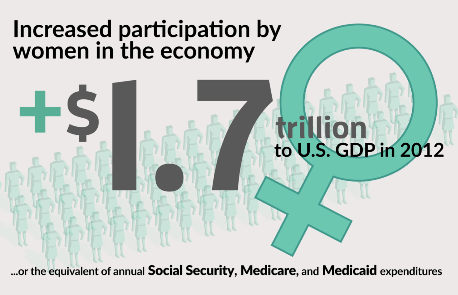
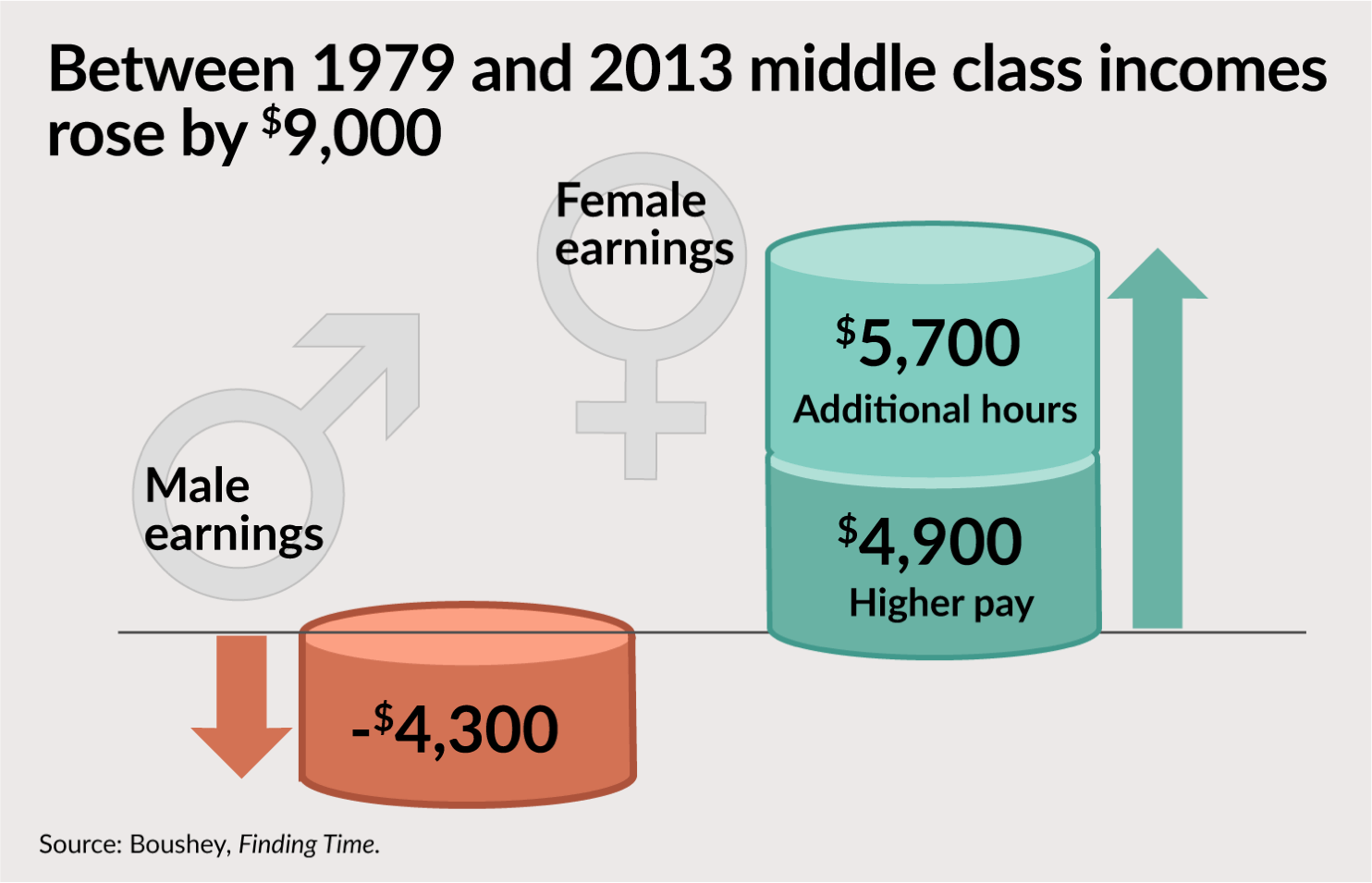
Since 1979, because of women’s added hours of work, our economy grew by 11 percent more than it would have otherwise. This is the equivalent to $1.7 trillion, equal to what we spend in a year on Social Security, Medicare, and Medicaid combined.

Women’s talents add to our nation’s productivity. And, their earnings boost family incomes.

Across the world, when women have access to education and jobs, we can see the positive effect on the economy. But, too often that power remains untapped. Economists estimate that the gender gap in employment leads to losses in GDP of 20 percent in Greece, Italy, and Japan to nearly 35 percent in the Gulf States and Iran. The International Labour Organization estimates that there are 865 million women who have the potential to contribute more to their economies. Most live in emerging or developing economies.

Here in the United States, we have solid evidence that women contributing their talents to American business and their family’s income has been good for our economy. This difference in how women spend their days changes everything. Women are not only their family’s caregiver, they are their family’s breadwinner.

The American Wife has become the American Worker. Only one in five children live in a family with a full-time, stay-at-home caregiver. Two out of every three mothers earns so much that she’s either the primary breadwinner or a co-breadwinner for her family. This is even though women earn only 79 on the male dollar—and women of color have an even larger pay gap.

We can all picture the “Leave it to Beaver” family. June’s at home caring for the Beav while Ward’s at work. Actually, can we? How many of you have even seen that show? How many see your family in that fictionalized portrait? Yep, that family’s experience is seriously outdated. Yet our workplace policies still presume that’s what a family looks like. They assume we all have a magical silent partner at home taking care of all of life while we’re at work. But that’s fantasy.

Caregiving—whether for a child or an aging parent—remains time-consuming and is increasingly expensive. To reconcile this, we need to rethink our nation’s basic labor standards and social protections. The United States stands with only Papua New Guinea in not having paid leave for mothers. And, I hear that Papua New Guinea is about to fix this!

California, New Jersey, Rhode Island and—soon—New York have universal, statewide paid family leave programs. In those states, a worker has the right to stay home—with pay—when they have a new child or to care for a seriously ill family member. Or when the worker herself is ill. On top of this, nearly three dozen places—five states, one county, 26 cities, and the District of Columbia (which, of course, is not a state)—have put in place the right for workers to earn paid sick days. That’s progress, but only for the lucky few who live in the right place.

Over 75 years ago, the first woman to lead a federal agency—Frances Perkins—helped craft into law two pieces of legislation that continue to define the rules that govern the boundaries between work and life. The Social Security Act gives us a set of insurance programs for when we cannot work, because we are a senior citizen, are too disabled to work, or when we’ve lost a job through no fault of our own. But we don’t have the same right to income support when we cannot work because we need to care for a family member for a few weeks  months. And, too often, those that have it earn the most. That’s not fair. To improve our economy, that needs to be fixed.

Every worker needs access to paid family and medical leave, including men. While women continue to do more care, men are increasingly stepping up and they’re realizing that it’s hard. In some surveys, men report more work-life conflict that women do.

The truth is, without the added hours of women, most families would have seen their incomes fall in recent decades. Women’s earnings have boosted family incomes, while also improving our overall economy through improving productivity. That’s why today’s workers also need predictable schedules and the right to talk to their boss about their schedule without fear of retaliation.

Putting sane rules on hours was another idea Mrs. Perkins championed. The Fair Labor Standards Act eradicated child labor and established the minimum wage and 8-hour workday. Recently, the Obama administration updated the overtime rules to cover an additional 4 million people.

This is a much-needed step forward. However, without a silent partner at home, chaotic or unpredictable schedules can wreak havoc on family life. And, it can mean that for an employee to be their most productive, they may need a little flexibility. With fewer than one in ten private sector employees having a union to help them negotiate schedules, most of us are on our own.

New rules that update our labor standards could fix this. Vermont and San Francisco are doing just that. They followed the lead of the United Kingdom and New Zealand, offering workers the right to request flexibility. And, San Francisco also added rules on predictability.

As many states and localities have recognized, the American Wife is the American Worker. That’s good for families and the economy.

We need new federal rules.

We can fix this.

The United States is and remains one of the richest nations the world has ever seen.

So, let’s do it.


Equitable Growth in Conversation: An interview with Claudia Goldin

“Equitable Growth in Conversation” is a recurring series where we talk with economists and other social scientists to help us better understand whether and how economic inequality affects economic growth and stability.
In this installment, Equitable Growth’s Executive Director and Chief Economist Heather Boushey talks with economist Claudia Goldin about the gender wage gap and some of its implications. Read their conversation below.


Heather Boushey: I want to focus on your work on the gender wage gap. Lots of us have been thinking about this for a long time and noticed that you have gotten a lot of attention in the press for your recent research on this, so I wanted to ask you some questions teasing out both what it is and what some of the implications are.

In your paper, “A Grand Gender Convergence: Its Last Chapter“—and I love the title of that—you argue that the gender wage gap cannot be explained by differences in productivity between men and women. Instead, when we look at occupations, we see that there is a price paid for flexibility in the workplace. And given what people are thinking about in terms of policy, that seemed like a really good place to start our conversation today. Can you tell me a little bit more about this result?

Claudia Goldin: So the key finding is that there is a gender wage gap. But the question is why? We know from lots of people’s work that we used to be able to squeeze a lot of the gap away due to differences in education—differences in your college major, whether you went to college or not, whether you have a Ph.D., an M.D., whatever. We were also able to squeeze a lot away on the basis of whether you had continuous work experience or not.

Today, we are not able to squeeze much away. In fact, women on average have more education than men. The quantities [of women with college degrees] are higher, and even the qualities [of degrees] aren’t that much different anymore. And the extent of past labor force participation is pretty high. Lifecycle labor force participation for women is very, very high. So we can’t squeeze that much away anymore.

What’s also really striking is that, given lots of factors such as an individual’s education level, many occupations have very large gender gaps and some occupations have very small gender gaps. Looking at occupations at the higher part of the income spectrum, which is also the higher part of the education spectrum — so occupations where about 50 or 60 percent of all college graduates are—we see that the biggest gaps are in occupations in the corporate and finance field, in law, and in health occupations that have high amounts of self-employment. And the smallest gaps are found in occupations in technology, in science, and in lots of the health occupations where there is a very low level of self-employment.

That’s sort of a striking finding.

Then when we dig deeper and look at particular occupations—in law, for example, and in the corporate and finance field—we see a couple of things. We see that differences in hours have very high penalties even on a per hour basis. Differences in short amounts of time off have very high penalties, unlike in other fields. And many of the differences occur at the event of or just after the event of first birth. So there is something that looks like women disproportionately, relative to men, are doing something different after they have kids.

When we look at men and women in the finance and corporate fields who haven’t taken any time off and among the women who don’t have kids, we find that the differences are really tiny. So those are the differences that are coming about, not surprisingly, from the fact that women are valuing predictability, and flexibility, and many other aspects of the job that many men are not valuing.

So, looking at data for the United States, we find that this change from being an employee, a worker, and a professional, to being an employee, a worker, a professional, and a parent has a disproportionate impact on women.

Now one might say, isn’t that because the United States has really lousy coverage in terms of parental leave policy, and in terms of subsidized daycare? Well, there are two very interesting papers, one for Sweden and one for Denmark. Both countries have policies that are just about the best in the world, and these studies, using these extraordinary cradle-to-grave data that they have, look at the widening in the — what men are getting versus women is occurring at — they can do an event study at that [having a child].

And women are moving into occupations that have more flexibility, but they are working fewer hours and getting less per hour. And the same sorts of things are going on even in countries that have incredibly good parental leave policies, subsidized daycare, schools that appear to us to be better, and what we think of as social norms that are better.

Boushey: One of the things that you found in your research that you haven’t mentioned yet is this idea that some workers are more substitutable—this idea that the industries with a high level of self-employment play some role in the gender pay gap. Could you explain that a little bit?

Goldin: Well, it would be very nice for us to go to each one of these occupations and take part in each one of these occupations and learn something about them. We can’t do that so instead we use the O*NET database, which gives us a lot of information about what goes on in these occupations.

And in O*NET, there are certain characteristics of the occupations that seem to map very nicely into aspects that would appear to be important, such as how predictable the job is, what the time demands are, whether you have to deal with clients, or whether work relationships are important.

And much of that is related to the issue about whether if an individual wants to leave work at 11 o’clock in the morning but do the same task at 11 o’clock at night, whether that’s severely penalized. That would be penalized if the individual can’t easily hand off work to someone else if it is needed at 11 a.m. That would be important if the fidelity of the information would be altered, if the client would feel that the individual wasn’t a very good substitute, and so on.

So using this information from O*NET, I find that the occupations that have the largest gender gaps are those that have the least predictability and the greatest time demands. And the occupations that have the smallest gender gaps are on the other side. It’s not necessarily causal, but it’s pretty good evidence that there is something going on.

And then I drill down deeper into particular occupations, such as the work that I have done on MBAs in the corporate and finance sector, and the longitudinal information that exists on lawyers. And finally, there’s a very interesting occupation that went through tremendous change during the 20th century and into the 21st century, and that’s pharmacy.

Pharmacists used to own their own businesses by and large, and they hired other pharmacists to work with them, often part-time. Many of these part-time workers were women, but there were few women who were owners. Well, ownership involves lots of responsibility, and as the owner, you are the residual claimant [the person with the last claim to the firm’s assets]. So in 1970 or so, women got about 66 cents on the male dollar in terms of pharmacy. Today, women working full-time full-year get 92 cents on the male dollar, uncorrected for any other differences and a lot more adding other relevant factors.

There are three things going on here. One is that there is no longer a lot of self-employment. Pharmacists by and large are not working for independent pharmacies anymore. They are working for big chains, national chains, regional chains, world chains. So the residual claimant now is the owner of the stock. There is professional management, and then there are just people who work there who are pharmacists.

The second thing is that there is very good use of IT. Every pharmacist now knows all the prescriptions that you have under your health plan, not just the ones that were filled in that pharmacy. And the third thing is that the drugs themselves are highly standardized by and large, so it isn’t that you are very attached to a particular pharmacist because they fill your prescriptions better or because they know you better. Pharmacists are highly paid professionals, but they are very good substitutes for each other.

Boushey: I’m glad you brought that study up, because I was going to ask you about it. My great uncle was a pharmacist, so I also just find it personally a fascinating example.

If you look at O*NET and the kinds of things that you are measuring, it seems like there are some cases where it seems very logical—especially in the case of pharmacists—that the substitutability is related to the profitability of the firm. It seems like a real strong business case.

Have you found in your research examples where perhaps not the substitutability but the job requirements around predictability or schedules may be more about keeping some workers out than they are about what’s good for the firm?

Goldin: Well, I’m all ears. (Laughter.)

Boushey: Yeah, I don’t know that I have answers there. I just think it begs the question. And I don’t know if you have thought about how to discern that difference in terms of —

Goldin: It’s that firms are leaving very large amounts of money on the ground. And so, if they are able to do that, they are able to pay for their taste for discrimination, then they can [discriminate]. And so that’s what one would look for, whether there are invaders standing at the gates. And if there aren’t, then they can do that and get away with it.

But the question is, where are the invaders that should be standing at the gates?

Boushey: And if part of what you have found is that a lot of this happens right after a child, that’s an invader of a different kind, perhaps.

Goldin: What’s interesting in the case of the MBAs is that it’s not right after the kid. It’s like two years later.

Babies are easier to take care of than 2-year-olds, and so it’s not that the firm then says, “Aha, we have one of those that has kids. We’ll just make certain that she doesn’t get the clients.” And one hears a lot of those stories, and those are the ones that the HR people are always talking about and making certain that people in their firm don’t do that—don’t have sexist paternalism, as it’s called.

But that doesn’t seem to be what is going on. I’m not doubting that there isn’t some of that, but what seems to be going on is that the individual tries and tries—in our data at least, in the Chicago Booth [School of Business] data—and eventually it’s just too much. There are too many demands, so they decide to scale back somewhat.

Boushey: Then I guess there are two questions. It sounds like it is that scaling back that causes the gender pay gap, right?. And what can we do about it?

Goldin: If a firm somehow believes, or it’s the case that right now, its production function is such that working 80 hours a week is worth a lot more than having two workers work 40 hours a week, then that produces non-linearities in pay and it leads to exactly what we are seeing. End of story.

Boushey: And on the policy side, it sounds like there isn’t a lot of incentive from the firm’s side to fix that

Goldin: No, there’s a lot of incentive on the firm’s side. If I’m paying someone more than twice as much to work 80 hours a week than I’m paying two people to work 80 hours a week, then I should think about ways of reducing my costs.

And if I am working people 80 hours a week and that leads people with skills, very expensive skills, to leave, then I should want to do something to keep them there and to figure out how to make certain that they aren’t working 80 hours a week.

I often hear how the CEO of a company has said, “We really want to keep our talent—women as well as men who don’t want to work 80 hours a week, who don’t want the pressure of being called up when they are at a soccer game with their kids, on a Sunday or a Saturday or an evening, or whatever.” The CEO will set down a policy to ensure that doesn’t happen, but then there are a lot of managers who don’t hear that or who claim they don’t hear that. So lots of firms hire HR people to go around and make certain that this is policed.

And these issues are present even in the military. Some time ago at a conference on workplace flexibility, Adm. Mike Mullen, former Chairman of the Joint Chiefs of Staff, essentially said “I’m having trouble doing it, and I’m the head of the entire military.”

So there are principal-agent problems that firms would like to rein in. So they are losing money.

Boushey: Yeah. Well, the federal government implemented a “right to request” policy in one of the agencies—I believe it was OPM, the Office of Personnel Management. I talked to them when they were starting to implement that and the folks we were talking to were super excited, and then they told me, “Oh, yeah, we had some problems with middle management actually implementing it.” And then they stopped the experimenting and I never heard about it again.

Goldin: Yeah.

Boushey: And I think it’s a real challenge how firms are making that connection between that profit motive that the big guys are thinking about and what’s actually happening.

Goldin: Right. But there are lots of firms that have what they call work-life balance, or work-family balance; where, if you work at 11 at night versus 11 in the morning, that’s perfectly fine with them.

I was talking with a very senior partner at a well-known consulting firm once and I asked, “Well, what do you do when clients [call people up at 11 p.m.]?” And she said, “I call up the clients and I say, I have staff and they are not your slaves.” Well. (Laughter.)

Boushey: Good for her.

Goldin: Good for her, and right. But let’s just say that there are cases in which we don’t want someone to have a perfect substitute. I do not want my president, for example, to turn around and say, “oh, by the way, I really don’t like this unpredictability business. You know? That little red button on the phone—every now and again, I say, you know, I’m really not here right now.” (Laughter.)

Because there are cases in which that person better be on 24/7 and that’s it. And we know that in the world of work, those people get higher pay—or, in the case of our president, just get better ratings.

So there are going to be cases in which individuals who are willing to work long hours, work unpredictable hours, be on call, whatever we want to call it, are going to get more. And they are not going to be substitutable. And information is not going to flow perfectly, with total high fidelity.

The question is, what fraction of the occupations in the economy are like that? And I think you and I would agree that the fraction is probably a lot lower than appears to be the case right now.

Boushey: So what should folks who are thinking about policy do about this? Is there a role for us, or is this just a business case? Do they all have to learn this lesson on their own, or is there something policymakers can do?

Goldin: Yeah, we have a policy. It’s called public schools. We’ve had it for a very, very long time. We have public schools that get out nationwide at about 2:30 or 3:00, that end sometime in June, that begin school at 5 years old or 6 years old. None of that was ever discussed as being the optimal way to run schools.

It is suboptimal with respect to individuals who have kids, because kids are not one- or two-year capital goods. Family leave policy is not the only thing that’s going to help families with kids, because the kids live, I hope, for many, many years after they are 2 years old. That’s the policy.

Boushey: I love it. That’s a fantastic way to end this interview, and something I will take with me in my travels here in Washington. Thank you so much, Claudia.

Goldin: Thank you.

This interview has been edited for length and clarity.

Garnering economic security is complicated for young families

Sara Gustoff, right, reads to her children Abigail, from left, Nathanael, Benjamin, and Jonah while at the kitchen table in their home in Des Moines, Iowa.

Overview

Over the past 40 years, women in the United States have played an increasingly important role in family economic well-being. Women have increased their levels of educational attainment and their participation in the labor force and have seen increases in pay. This transformation in how women spend their days means that most families must figure out how to make do without a full-time, stay-at-home caregiver.

While conflicts between the demands of work and caregiving are now commonplace, families too often are left on their own to cope, without the support of sufficient social infrastructure—such as affordable child care and elder care, paid time off for medical and family leave, and the flexible work hours—and macroeconomic policies that would reduce unemployment, increase wages, and encourage full employment. These findings are detailed in Heather Boushey’s recently released book, “Finding Time: The Economics of Work-Life Conflict,” which explores how women’s increased hours of work over the past four decades helped American families maintain economic security.

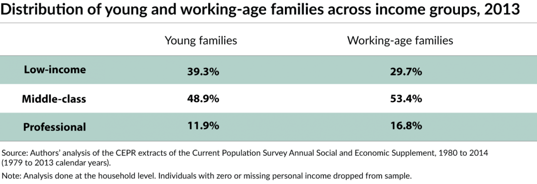
In this issue brief, we unpack women’s role in helping stabilize family incomes for a specific subset of the U.S. population: young families, or families where at least one person is above the age of 16 and everyone is under the age of 35. Using data from the Current Population Survey, we chronicle how family incomes changed between 1979 and 2013 for young low-income, middle-class, and professional families. Specifically, we decompose the differences in male earnings, female earnings from greater pay, female earnings from more hours worked, and other sources of income over this time period.

Download File
Garnering economic security is complicated for young families (pdf)

Read the full pdf in your browser

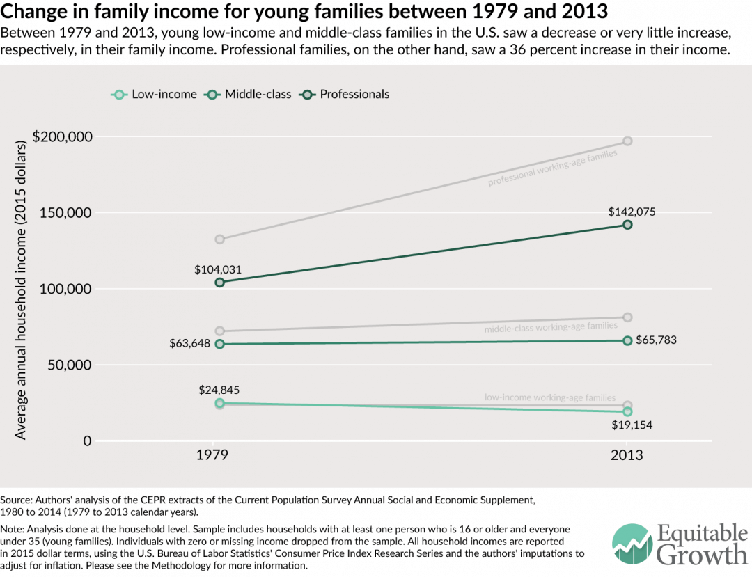
We find that even though women in young families have increased their hours of work as much as women in the working-age families in our issue brief “Women have made the difference for family economics security,” these young families have seen less income growth.

Here are our key findings:

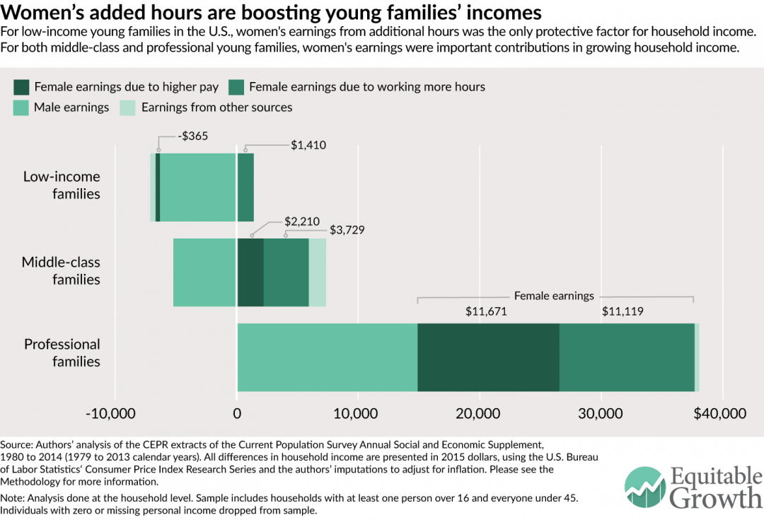
  • Even as women’s hours increased, declining male earnings pulled down family income in both low-income and middle-class young families. Among young low-income families, income fell by 22.9 percent over that time period, while among young middle-class families, income only grew by 3.4 percent.
  • Between 1979 and 2013, women’s added hours of work boosted young families’ income across income groups. For low-income families, women’s added hours were the only growth factor. In both middle-class and professional young families, women’s higher earnings from increased pay also bolstered family incomes.
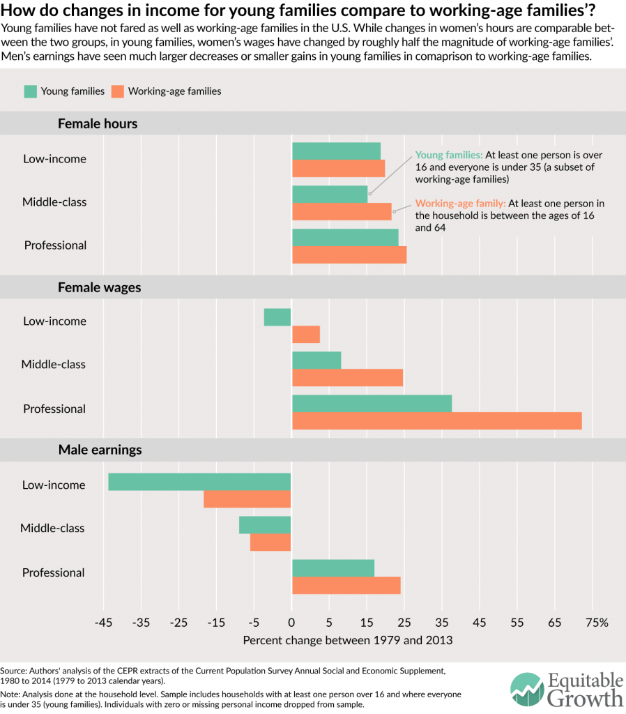
  • While the work hours of women in young families increased at similar rates to the hours of women in working-age families across all three income groups, young families saw much smaller growth in women’s wages and larger losses or smaller gains in male earnings compared to working-age families.

The economic state of young workers

Despite recent improvements in the U.S. labor market, young workers continue to face tough conditions. This past March, for example, the unemployment rate for all people over the age of 16 was 5.0 percent, but was 8.4 percent for young workers (ages 20 to 24). The challenges, however, go beyond relatively high unemployment and underemployment (compared to older workers) and include slow wage growth, limited opportunities to move up the job ladder, and, for those that have not been able to find a firm foothold in the job market, the long-term scarring of their earnings potential.

Higher unemployment among younger workers is due to a number of factors, not all of which are bad. We expect that young workers will change jobs more often—ideally, transitioning between jobs to find better offers—as they build their careers and grow their earnings. To the extent that young workers’ higher unemployment is due to spending more time seeking jobs or moving to a different city, this is not necessarily bad.

But there also are not-so-good reasons for higher unemployment. Young workers are often first-time job seekers with limited work experience, which makes them more likely to be passed over in hiring decisions. Even once they are hired, they are typically the most junior employees and thus most susceptible to being laid off or let go when their firms run into trouble.

The Great Recession of 2007–2009 created a host of challenges for young workers: Those who entered the labor market at that time, couldn’t find their footing, and then were often overlooked in favor of “fresh” workers in later years. Research by economists Giuseppe Moscarini at Yale University and Fabien Postel-Vinay at University College London finds that during the Great Recession, many workers became trapped in low-wage jobs, which they describe as the job ladder “shutting down.” On top of this, for many young workers who earned a college degree, the added burden of increasing student debt loads delayed steps in the traditional economic lifecycle, among them homeownership, car ownership, and even marriage.

Economic struggles are compounded for the nearly half of young families with children. In 2013, almost half (43.7 percent) of young families had a child under age 18 present in the home. The higher up a young family is on the income ladder, the less likely they are to have a child at home. Among young professional families, only 22.6 percent have a child at home, compared to 37.7 percent among middle-class families and 57.6 percent among low-income families.

Young families struggle with how to address work-life conflict within the context of this tough labor market. As Heather Boushey documents in her book, “Finding Time: The Economics of Work-Life Conflict,” families over the past four decades have relied on the added hours and earnings of women to boost income. Women’s increased participation in the labor force has been an effective coping mechanism amid the shifting fortunes for male workers in the U.S. economy over this period, directly contributing to family economic security. But this can be a tough strategy without policies to help address the day-in, day-out conflicts between work and family life. This can be even harder for young workers who are least likely to have built up reserves of sick or vacation time or may be more vulnerable to layoffs.

This issue brief extends the analysis in “Finding Time” and explores what this looks like specifically for young families up and down the income ladder. Using data from the Current Population Survey, we calculate how family income has changed between 1979 and 2013 for low-income, middle-class, and professional families who are “young”—where at least one person is above the age of 16 and everyone in the household is 35 years old or younger. (See Box.) We decompose these changes over time into differences in male earnings, female earnings from more pay, female earnings from more hours worked, and other sources of income, which include Social Security and pensions, which are minimal given the age of workers in these families.

Between 1979 and 2013, young families saw comparatively small gains—and in the case of low-income families, large losses—in family income. When we break down the changes in household income, we find that over those 34 years, for low-income young families, the only positive contribution to income was the added earnings women received by working more hours. For young middle-class and professional families, female earnings (from both more pay and hours) have been crucial in mitigating steep drops or even smaller increases, respectively.

Defining income groups and young families

The analysis in this issue brief follows the same methodology presented in “Finding Time.” For ease of composition, we use the term “family” throughout the brief, even though the analysis is done at the household level.

In this issue brief, we refer to what we call “young” families and compare their experiences to “working-age” families. A working-age family (the subject of an earlier issue brief) is one where at least one person in the household is between the ages of 16 and 64. Young families are a subset of these working-age families: Young families are those that have at least one person over the age of 16 and where everyone is under 35 years of age.

We split households in our sample into three income groups:

  • Low-income households are those in the bottom third of the income distribution, earning less than $25,440 per year in 2015 dollars.
  • Professional households are those in the top fifth of the income distribution who have at least one household member with a college degree or higher. These households have an income of $71,158 or higher in 2015 dollars.
  • Everyone else falls in the middle-class category.

Table 1 breaks down the share of young families (a subset of these working-age families) across the three income groups in 2013. Young families are more likely than working-age families to be low-income.

Table 1

Setting some context

Before focusing on the changes in family income, let’s first set some broad context for the changes in family economics between 1979 and 2013.

How did income change for young families?

Between 1979 and 2013, young low-income families lost income, middle-class ones experienced small gains, and professionals saw their income soar. These trends follow those more generally for working-age families. The key difference between young and working-age families, however, is that young families’ income levels are lower than those of working-age families more generally. (See Figure 1.)

Figure 1

Young families have seen the same rising inequality that has affected families overall. In 1979, low-income young families had an average annual household income of $24,845 in 2015 dollars. Between 1979 and 2013, these families saw their income drop by 22.9 percent, down to $19,154. This is a significant decrease; between 1979 and 2013, low-income working-age families’ income fell only by 2.0 percent on average. Over the same time period, young middle-class families’ income stalled. In 1979, young middle-class families had an average household income of $63,648, which had grown only slightly—by 3.4 percent—to $65,783 in 2013. Young professional families, however, saw their income rise 36.6 percent, going from $104,031 in 1979 to $142,075 in 2013.

Inter-group disparities in family income are not only an indication of widening inequality but also may indicate that “filtering down” is underway. Recently, because there have not been enough jobs to employ all the young workers who need a job, those with a college degree (some of which are categorized as professionals in our analysis) have been scooping up a disproportionate share of the jobs available—even those jobs that do not require a college degree. This crowds out young workers without a college degree (most of whom fall into either our middle-class or low-income groups), making it much harder for less-educated workers to find suitable employment. Instead, they must either accept an even lower-paying job or exit the labor market completely. This might shed some light on why young low-income families have seen larger losses in income.

How did women’s working hours change in young families?

Between 1979 and 2013, across all three income groups, women in young families increased their working hours. In 1979, on average, women from young low-income households worked 662 hours annually (about 13 hours per week), and by 2013, their hours had grown by 23.0 percent to 814 (or 16 hours per week). Over this same time period, women from young middle-class families, on average, grew their annual hours by 19.8 percent, from 1,109 in 1979 to 1,328 in 2013 (or from 21 hours per week to 26 hours per week). Similarly, women in young professional families saw a 27.4 percent rise in their hours of work. (See Figure 2.)

Figure 2

The shift in hours is virtually identical across young and working-age women in professional families, but the trends differ by age within low-income and middle-class families. In middle-class families, women in working-age families put in more hours than those in young families. This could be due to more women in young middle-class families being in school rather than working. Yet within low-income families, women in young families are slightly more likely to have a paying job than are women in working-age families, and this was true in both 1979 and 2013.

Decomposing the changes in young families’ income

Figures 1 and 2 show that between 1979 and 2013, hours of work for women in young families increased across all income groups, yet family income has not increased commensurately across all three groups. To understand what’s going on, we decompose the changes in young families’ average household income between 1979 and 2013 into male earnings, female earnings, and income from other non-employment-related sources, which include Social Security and pensions. Specifically, we divide female earnings into the portion due to women earning more per hour and the portion due to women working more per year. To calculate female earnings stemming directly from the additional hours worked, we take the difference between 2013 female earnings and the hypothetical earnings of women if they earned 2013 hourly wages but worked the same hours as women did in 1979. (For more on how we did this calculation, please see our Methodology.)

We find that within young families across the income spectrum, women’s contributions, particularly from more working hours, have been the most important factor in boosting family incomes. Yet incomes have not risen in tandem, as both men’s earnings in low-income and middle-class families pulled down family income. Without women’s added hours and higher earnings, family income would have fallen, all else being equal. (See Figure 3.)

Figure 3

Between 1979 and 2013, young low-income families saw their income fall sharply. Most of this decline is due to the drop in men’s earnings—a loss of $6,305—although women’s earnings per hour also fell, reducing income by $365. Within young low-income families, the only positive contribution to household income was the added work hours of women, which boosted average annual income by $1,410.

Over this same period, in young middle-class families, average annual household income grew by more than $2,000, even though male earnings dragged family income down by $5,210. The only reason middle-class families saw any income gains was because of increases in women’s earnings, both in terms of higher pay per hour and more hours of work. Women’s earnings from more work hours accounted for the largest component of the gain, adding $3,729 to average annual income. The second-largest component was women’s earnings from higher pay, which added $2,210. Income from other (non-employment) sources also helped boost the incomes of young middle-class families.

Young professional families experienced significant growth in average income. Combined, women’s higher earnings from higher pay and additional hours of work boosted family income by $22,790, close to 60 percent of the total change. In stark contrast to men in young low-income or middle-class families, men in young professional families saw their earnings rise—adding $14,886 to family income. Young professional families had a relatively negligible positive change in other sources of income.

How does the experience of young families compare to working-age families?

Young families have not fared as well as working-age families more generally. When we look at the changes to family income between 1979 and 2013 for young and working-age families side by side, the challenges facing young families is put in sharp relief. Specifically, we compare the percent change in women’s hours and wages—both of which are components used in calculating women’s earnings due to more hours worked—and men’s earnings for young and working-age low-income, middle-class, and professional families. (See Figure 4.)

Figure 4

Across income groups, women from young and working-age families have seen similar rates of increase in their working hours, a fact that we saw earlier in Figure 2. But despite these similarities, the wages of women from young families did not grow nearly as much as the wages of women from working-age families. In fact, in low-income young families, women’s wages fell by 5.6 percent, compared to 8.1 percent growth in women’s wages for low-income working-age families. For the middle-class and professional income groups, young families saw much smaller gains—roughly half—in women’s wages than working-age families.

What is also striking is that across the board, men had worse earnings outcomes in young families in comparison to working-age families. At the bottom of the income ladder, men from young families saw their earnings fall by 43.8 percent, while the earnings of men from working-age families only fell by 20.4 percent. Middle-class men’s earnings for young and working-age families dropped by relatively similar percentages (11.7 percent and 9.0 percent, respectively). At the top, men from young professional families saw a 21.5 percent increase in their earnings compared to a 27.9 percent increase in men’s earnings in working-age professional families.

Conclusion

Across income groups, women’s increased work hours and—for all but low-income families—rising pay have helped young families secure their income. When we compare their changes in family income between 1979 and 2013, young families are much worse off than working-age families, seeing greater losses and smaller gains in women’s wages and men’s earnings across the board.

So while women’s earnings from both more pay and hours have made a tangible positive difference for young families, it is simply not enough to strengthen their economic security. That’s why policies that would reduce unemployment, increase wages, and encourage full employment for young workers are essential. And when the labor market is weak, ensuring that safety net programs adequately support young workers and their families is an important way to give them an equitable chance to improve their futures.

Further, with women’s added hours of work being so important to family economic well-being, the reality is that young families and working-age families alike need access to policies to help them address work-life conflicts. Nearly half of young families have a small child at home and are balancing the needs of parenting young children with holding down a job. They need access to the same basket of policies other workers need, including paid sick days, paid family and medical leave, and access to safe, affordable, and enriching child care. Many young people are also trying to navigate a work schedule with earning an educational degree, and policies such as those that promote predictable schedules can help them invest in their future while holding down a job to make ends meet.

Heather Boushey is the Executive Director and Chief Economist at the Washington Center for Equitable Growth, and the author of the book “Finding Time: The Economics of Work-Life Conflict” from Harvard University Press. Kavya Vaghul is a Research Analyst at Equitable Growth.

Acknowledgements

The authors would like to thank John Schmitt, Ben Zipperer, Dave Evans, Ed Paisley, David Hudson, and Bridget Ansel. All errors are, of course, ours alone.

Methodology

The methodology used for this issue brief is identical to that detailed in the Appendix to Heather Boushey’s “Finding Time: The Economics of Work-Life Conflict.” wanted to find out from you whether I also need to include these cutoffs. Thanks!s adequately support young workers and their fa

In this issue brief, we use the Center for Economic and Policy Research extracts of the Current Population Survey Annual Social and Economic Supplement for survey years 1980 and 2014 (calendar years 1979 and 2013). The CPS provides data on income, earnings from employment, hours, and educational attainment. All dollar values are reported in 2015 dollars, adjusted for inflation using the Consumer Price Index Research Series available from the U.S. Bureau of Labor Statistics. Because the Consumer Price Index Research Series only includes indices through 2014, we used the rate of increase between 2014 and 2015 in the Consumer Price Index for all urban consumers from the Bureau of Labor Statistics to scale up the Research Series’ 2014 index value to a reasonable 2015 index estimate. We then used this 2015 index value to adjust all results presented.

For ease of composition, throughout this brief we use the term “family,” even though the analysis is done at the household level. According to the U.S. Census Bureau, in 2014, two-thirds of households were made up of families, defined as at least one person related to the head of household by birth, marriage, or adoption.

We divide our sample into three income groups—low-income, middle-class, and professional households—using the definitions outlined in “Finding Time” and detailed in the box presented in the analysis above. For calendar year 2013, the last year for which we have data at the time of this analysis, we categorized the income groups as follows:

  • Low-income households are those in the bottom third of the size-adjusted household income distribution. These households had an income below $25,440 (as compared to $25,242 and below for 2012). In 1979, 28.3 percent of all households were low-income, increasing to 29.7 percent in 2013. These percentages are slightly lower than one-third because the cut-off for low-income households is based on household income data that includes people of all ages, while our analysis is limited to households with at least one person between the ages of 16 and 64. The working-age population (ages 16 to 64) typically has higher incomes than older workers, and as a result, the working-age population has somewhat fewer households that fall into this low-income category.
  • Professionals are those households that are in the top quintile of the size-adjusted household income distribution and have at least one member who holds a college degree or higher. In 2013, professional households had an income of $71,158 or higher (as compared to $70,643 or higher in 2012). In 1979, 10.2 percent of households were considered professional, and by 2013, this share had grown to 16.8 percent.
  • Everyone else falls in the middle-class category. For this group, the household income ranges from $25,440 to $71,158 in 2013 (as compared to $25,242 to $70,643 in 2012); the upper threshold, however, may be higher for those households without a college graduate but with a member who has an extremely high-paying job. This explains why within the middle-income group, the share of households exceeds 50 percent: The share of middle-income households declined from 62 percent in 1979 to 53.4 percent in 2013.

Note that all cut-offs above are displayed in 2015 dollars, using the inflation-adjustment method presented earlier.

In our analysis, we limit the universe to people with non-missing, positive income of any type. This means that even if a person does not have earnings from some form of employment but does receive income from Social Security, pensions, or any other source recorded by the CPS, they are included in our analysis. Additionally, we limited our sample to young families—or households where at least one person is older than 16 and everyone is under the age of 35.

These data are decomposed into income changes between 1979 and 2013 for low-income, middle-class, and professional families. The actual household income decomposition uses a simple shift-share analysis to find the differences in earnings between 1979 and 2013 and calculate the extra earnings due to increased hours worked by women.

To do this, we first calculate the male, female, and other earnings by the three income categories. To calculate the sex-specific earnings per household, we sum the income from wages and income from self-employment for men and women, respectively. The amount for other earnings is derived by subtracting the male and female earnings from total household earnings. We average the household, male, female, and other earnings by each income group for 1979 and 2013 and take the differences between the two years to show the raw changes in earnings by each income group.

To find the change in hours, for each year, by household, we sum the total hours worked by men and women. We average these per-household male and female hours, by year, for each of the three income groups.

Finally, we calculate the counterfactual earnings of women. We use the 2013 earnings per hour for women and multiply it by the 1979 hours worked by women. Finally, we subtract these counterfactual earnings from the female earnings in 2013, arriving at the female earnings due to additional hours.

One important point to note is that because of the nature of this shift-share analysis, the averages don’t exactly tally up to the raw data. Therefore, when presenting average income, we use the sum of the decomposed parts of income. While economists typically show median income, for ease of composition and the constraints of the decomposition analysis, we show the averages so that the data are consistent across figures. Another important note is that we make no adjustments for changes over time in topcoding of income, which likely has the effect of exaggerating the increase in professional families’ income relative to the other two income groups.

Another interactive look at changes in U.S. labor force participation

Last week we published an interactive graph showing trends in U.S. labor force participation since 1975, using data from the Current Population Survey. While that graph lets you select which time period you want to look at, we thought it might be informative to be able to pick which age group you want to look at. That’s what the interactive below allows you to do.

Select an age bracket and see trends in the share of U.S. workers who are:

• Employed part-time or full-time
• Officially unemployed
• Disabled
• In-home caregivers
• Students in school
• Retired

History of Labor Participation by Age Bracket
A history of labor market participation by age bracket
Choose an age bracket to see how labor participation within that bracket has changed over time. Click on an area of the chart to isolate that category.
Recessions are shaded, red lines indicate a major change to the CPS survey.
Note: This chart is updated monthly. Data is from the Census Bureau's Current Population Survey. Basic monthly data are used and all months are averaged together for each year. The survey was revised in 1989 and 1994; changes to both question wording and survey weights result in discontinuities in these years that may not be attributable to real changes in the economy. Recession data from: Federal Reserve Bank of St. Louis, NBER based Recession Indicators for the United States from the Period following the Peak through the Trough [USREC], retrieved from FRED, Federal Reserve Bank of St. Louis https://research.stlouisfed.org/fred2/series/USREC, March 1, 2016.

Methodology

The data assembled span three versions of the Current Population Survey, with new surveys being instituted in 1989 and 1994. All three surveys feature a labor force participation item that is generated based on responses to a series of yes/no questions on the survey. This variable is called ESR, LFSR, and PEMLR, respectively, on the three versions of the survey. A second variable—called major activity, or MAJACT, on the first two surveys and PENLFACT on the post-1994 survey—was used to distinguish between certain categories of non-labor force respondents. Finally, a question on total hours worked was used to distinguish full-time workers from part-time workers.

The results are fairly consistent across surveys for certain age groups but there are important discrepancies. Most notably, the pre-1989 survey did not allow respondents to specifically identify themselves as retired. Instead, the “other” category included retirees. The wording and question order of the 1989-1993 survey appears to bias respondents in favor of choosing “carer” over “retired,” so another break in the retired series is evident in 1994. Minor changes in the survey may also have contributed to the uptick in respondents identifying as “disabled” in the most recent version of the survey.

This project’s github includes the Python code that was used to analyze the raw monthly CPS data, including our survey-weighting procedure and all coding decisions made.

An interactive history of U.S. labor force participation

If you want to know how the labor market has changed over time, you usually look at the unemployment rate or maybe the employment-to-population ratio. But while those summary statistics are important, they don’t tell us about what people outside the labor force are doing. Are they in school? Acting as a primary caregiver? Disabled? Retired from the workforce?

The chances a worker is in any of those roles at a specific age during their life has changed quite a bit over the years. Inspired by Matt Bruenig of Demos, we looked at the trends in labor force status by age since 1975, using data from the Current Population Survey.

The interactive graph below shows the share of U.S. workers at different ages who are:

  • Employed part-time or full-time
  • Officially unemployed
  • Disabled
  • In-home caregivers
  • Students in school
  • Retired
History of Labor Participation Interactive
An interactive look at participation in the labor force by age
Click an area on the chart to isolate that category. Slide along the GDP growth graph under the chart to look at a different time period.
Slide to pick a year (recessions are shaded), red lines indicate a major change to the CPS survey.
Note: This chart is updated monthly. Data is from the Census Bureau's Current Population Survey. Basic monthly data are used and all months are averaged together for each year. The survey was revised in 1989 and 1994; changes to both question wording and survey weights result in discontinuities in these years that may not be attributable to real changes in the economy. GDP data from: US. Bureau of Economic Analysis, Gross Domestic Product [GDP], retrieved from FRED, Federal Reserve Bank of St. Louis https://research.stlouisfed.org/fred2/series/GDP. Recession data from: Federal Reserve Bank of St. Louis, NBER based Recession Indicators for the United States from the Period following the Peak through the Trough [USREC], retrieved from FRED, Federal Reserve Bank of St. Louis https://research.stlouisfed.org/fred2/series/USREC, March 1, 2016.


Methodology

The data assembled span three versions of the Current Population Survey, with new surveys being instituted in 1989 and 1994. All three surveys feature a labor force participation item that is generated based on responses to a series of yes/no questions on the survey. This variable is called ESR, LFSR, and PEMLR, respectively, on the three versions of the survey. A second variable—called major activity, or MAJACT, on the first two surveys and PENLFACT on the post-1994 survey—was used to distinguish between certain categories of non-labor force respondents. Finally, a question on total hours worked was used to distinguish full-time workers from part-time workers.

The results are fairly consistent across surveys for certain age groups but there are important discrepancies. Most notably, the pre-1989 survey did not allow respondents to specifically identify themselves as retired. Instead, the “other” category included retirees. The wording and question order of the 1989-1993 survey appears to bias respondents in favor of choosing “carer” over “retired,” so another break in the retired series is evident in 1994. Minor changes in the survey may also have contributed to the uptick in respondents identifying as “disabled” in the most recent version of the survey.

This project’s github includes the Python code that was used to analyze the raw monthly CPS data, including our survey-weighting procedure and all coding decisions made.

Equitable Growth in Conversation: An interview with David Card and Alan Krueger

“Equitable Growth in Conversation” is a recurring series where we talk with economists and other social scientists to help us better understand whether and how economic inequality affects economic growth and stability.
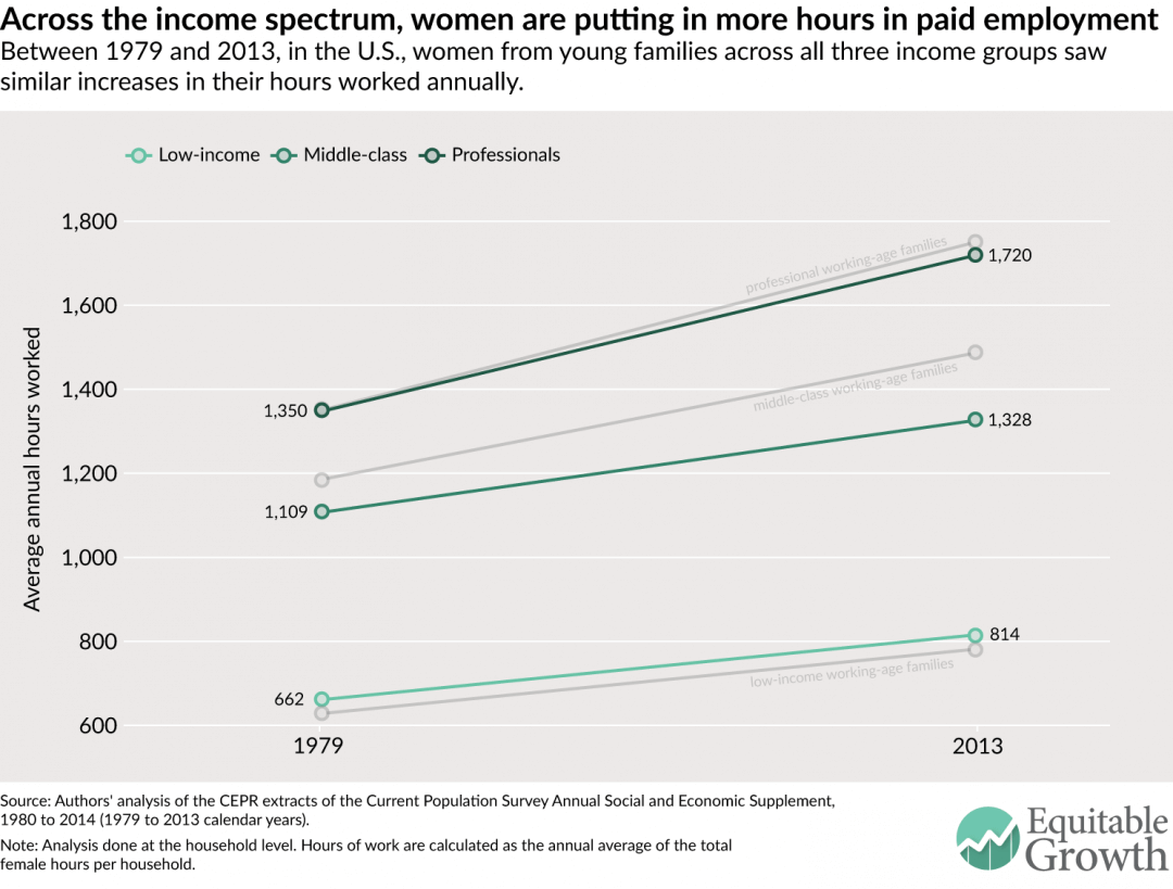
In this installment, Equitable Growth Research Economist Ben Zipperer talks with economists David Card and Alan Krueger. Their discussion touches on the origins of empirical techniques they advanced, how the United States is falling behind when it comes to data, and two conflicting threads of contemporary economic theory.

Read their conversation below.


Ben Zipperer: A common theme in both of your work involves isolating specific interventions or plausibly exogenous changes in the phenomena you’re studying, say in the case of your famous study comparing restaurants in New Jersey and Pennsylvania after a minimum wage increase. What kind of challenges did you face early on in that research—in the days before words or phrases like “research design” and “natural experiment” were kind of ubiquitous terms in the field of economics?

And then also, can you talk a little bit about the influence of the quasi-experimental approach on labor economics today and maybe the field of economics as a whole?

David Card: There are several origin stories that meet sometime in the late ’80s, I would say, in Princeton. One part of the origin story would be Bob LaLonde’s paper on evaluating the evaluation methodologies. So, in the 1970s, if you were taking a class in labor economics, you would spend a huge amount of time going through the modeling section and the econometric method. And ordinarily, you wouldn’t even talk about the tables. No one would even really think of that as the important part of the paper. The important part of the paper was laying out exactly what the method was.

But there was an underlying current of how believable are these estimates, what exactly are we missing. And some of that came to the fore in LaLonde’s paper.

He was a grad student at Princeton in the very first cohort that I advised: He was actually a grad student when I was a grad student, but he was a couple years behind me.  Then I was his co-adviser with Orley Ashenfelter. And in the course of doing that work, it became pretty obvious that these methods were very, very sensitive: If you played around with them, you got different answers.

The impetus of that paper was some work that Orley and I were asked to do evaluating the old CETA programs. There were a bunch of different methods that were around and they would give very different answers. So Orley had the idea of setting Bob on that direction and that really evolved that way.

So that was one part of the origin story. Another part was the move from macro-type evidence to micro evidence. There was growing appreciation of that. And the first person that I saw really use the phrase “natural experiment” was Richard Freeman.

Alan Krueger: That’s who I learned it from, too. Richard always had an interest in evidence-based natural experiments. He was an enormous fan of the work by LaLonde; also, the paper Orley did in JASA [the Journal of the American Statistical Association] on the negative income tax experiment. Richard always had a soft spot for natural experiments. But I think he used the term differently than we would.

He applied it to big shocks. So to him, the passage of the Civil Rights Act was a natural experiment. The tight labor market in the 1960s was another natural experiment. I think the way he viewed it was a bit different from the way it started to get applied, which was that the world opened up and made a change for some group that could be viewed as random. When Josh Angrist and I looked at compulsory schooling, we looked at a small change.  The natural experiment was just being born on one side or the other of the threshold for starting school, which then affected how many years of education you ultimately got because of different compulsory schooling laws and students would reach the minimum schooling age in different grades.

But that’s where I first heard the term.

Card: Right. And you mentioned research design. I remember Alan was an assistant professor and I was a professor at Princeton and Alan sat next to me. And he, for some reason, got a subscription to the New England Journal of Medicine. (Laughter.) And —

Zipperer: Intentionally?

Krueger: Yeah. I loved reading the New England Journal of Medicine.

Card: Yeah. And the New England Journal would come in every week, so there was a lot of stuff to read. And the beginning of each article would have “research design.”

Krueger: And “methods.”

Card: Yes, and if you’ve never seen that before and you were educated as an economist in the 1970s  or 1980s, that just didn’t make any sense. What is research design? And I remember one time I said, “I don’t think my papers have a research design.”

And so that whole set of terms entered economics as a result of those kinds of changes in orientation. But I would say that another thing that happened was that Bob LaLonde got a pretty good job and his paper got a lot of attention. And then Josh Angrist, again following up a suggestion from Orley to look at the Vietnam draft—that paper got a lot of attention. And it looked like there was a market, in a way, for this new style of work. It’s not like we were trying to sell something that no one wanted. There was actually a market out there generally, in the labor economics field, at least.

Krueger: There was, but there was also resistance. (Laughter.)

I agree with everything David said. The other thing—which I think helped to support this, although maybe it gets overrated—is that data became more available, and big datasets like the Census were easier to use.

Historically, when the 1960 Census microdata first became available, Jacob Mincer used it and had an enormous impact. And I think the fact that we were inventorying more data meant that if you wanted to look at a natural experiment – for example, a change in social security benefits which affected one cohort and not another —  the data were out there to do it.

I think another thing — which was a bit new when we did it for our American Economic Review article on the minimum wage — was to go out and collect our own data when we saw the opportunity to study a natural experiment. But in other situations the fact that there were just data out there to begin with, I think, helped this movement.

Card: Yeah. That was the case with my Mariel Boatlift paper. It was written a little bit before we started working on minimum wages. And in that case, it just so happened that the Outgoing Rotation Group files were available starting in 1979. And so, with those files, it was fairly straightforward to do an analysis of what affected even the Miami labor market.

And in retrospect there’s a new paper by George Borjas flailing around trying to overturn the results in my paper. But in truth, if somebody had been on the ground in Miami in 1980 and gotten their butts in gear, there would have been so much more interesting stuff to do.

For instance, when Hurricane Andrew happened, people actually convinced the CPS to do a survey or supplement, right?

Krueger: Yes.

Card: So, I think the whole, not just the profession, but even maybe the government, has become a little bit more aware of the importance of really strategically moving resources around and collecting data.

And now the administrative data is available for some things as well.

Zipperer: Speaking of data access, how important do you think it is now for work on the research frontier of labor economics, say, to have administrative data access, or access to often-restricted-access datasets? Is the United States positioned as a leader in this? Or are we paling in comparison to other countries?

Card: Well, we’ve got a lot of disadvantages. One problem is that we don’t have a centralized statistical agency. And so you’ll forever run into someone who wants to do a project and they’re not able to do it because there’s a bureaucratic obstacle to using this particular dataset or that particular dataset.

So for example, matching the LEHD [Longitudinal Employer-Household Dynamics] data to the Census of manufactures or the Census of firms. That would be a natural thing to do, but not that easy to do. If it was one statistical agency, we would have a lot more ease.

And then the laws of the United States—not just the federal but then the state laws—governing access to, say, the UI [unemployment insurance] files. Partially, those are available to the Feds when they’re constructing the LEHD data or other types of datasets, but they’re not available to individual researchers.

Although Alan and I have both used, for example, data from New Jersey. So individual researchers can, in some cases, contact the state and get some help. But that often requires some combination of a person on the other side who actually wants to answer the phone and talk to you, and maybe some resources.

Krueger: Yes, so I would say we’re behind other countries in terms of administrative datasets. We’ve long been behind Scandinavia, which has provided linked data for decades. And we’re now behind Germany, where a lot of interesting work is being done.

And it’s unfortunate because we did lead the world, I would say, in labor force surveys. The rest of the developed world copied our labor force survey and copied our practice of making the data available for researchers to use.

It’s much more cumbersome, bureaucratic, and idiosyncratic here to get access to the administrative data. And I don’t think that’s good for American economists or for studies of the economy.

And it’s going to make it much harder to replicate work going forward. And that’s unfortunate because I think a strength in economics has been the desire to replicate results.

Card: But I think it is absolutely critical for front-line research in the field to have access to some kind of data. Either you get access to administrative data through personal connections like a lot of people do. Or there are certain countries that make it available, like Germany, for instance—I’ve done a lot of work there—or Portugal. Or like Alan has done where he’s used some of the resources available at Princeton to do some specialized surveys and connect the responses with the administrative data. That’s probably the frontier at this point. But that’s not going to be a thing that a typical person can do very easily.

Krueger: And we haven’t caught up in terms of training students to collect original survey data. I’ve long thought we should have a course in economic methods—going back to the New England Journal of Medicine—and cover the topics that applied researchers really rely upon, but typically are forced to learn on their own. Index numbers, for example. Or ways of evaluating whether a questionnaire is measuring what you want it to measure. And survey design, sampling design and the effect of non-response bias on estimates.

These are topics that other social science fields often teach and we just take for granted that students know it. And there’s a lot of work that’s being done, especially in development economics, on implementing randomized experiments, which I think is a net positive. But there’s also a lot of noise being produced. And I think having more training in terms of data collection, survey design, experimental design, would be helpful for our field.

Zipperer: You mentioned randomized experiments. What are your views on the pluses and minuses of what seem to be a variety of different empirical approaches now common in economic research, such as randomized experiments, actually conducting an experiment? Or a quasi-experimental approach, compared to say, a more model-centric approach? Or even more recent kinds of data mining techniques that let the data tell us the research design?

Card: I would say, and I think Alan would probably agree with me, that at the end of the day, you probably want to have all those things if possible. And each of them has some strengths and some weaknesses.

The strength of a randomized controlled trial is the ability to say you’ve got this treatment and this control group and it’s random. So that means that you’re internally consistent. The weakness is that the set of questions you can ask and the context in which you can ask those questions is often very contrived.

So the one extreme is the lab experiment, where you’re getting a bunch of students and you’re asking them to pretend that they’re two sides of a bargaining table or something similar. And by changing the way you set the protocols for those experiments, as people that work in that field are aware, you can get somewhat different answers. To some extent, the criticisms of psychology that you would see played out in the newspapers recently has a lot to do with those difficulties. It’s not just how you read the script but how you set up the lab and everything else that kind of matters.

So the great advantage of a quasi-experiment or natural experimental like minimum wage is that it’s a real intervention. It’s real firms that are all affected. You get part of the general equilibrium effect. That’s pretty important for understanding the overall story. The disadvantage is that someone can always say, well, it isn’t truly random. And the number of units might be small. So you might only have two states. At some abstract level, there’s only two degrees of freedom there. And so that’s a problem.

And then there’s a third set of problems, which I’ve alluded to before, which is the types of questions that you can ask. And this is where my former colleague, Angus Deaton, is well-known for his vitriolic criticism of RCTs in development economics.

And I think one interpretation of his concern is the set of questions that can be asked are really so small, relative to the bigger questions in the field. Now that isn’t always the case but that is a concern.

Krueger: Yes, I would just add that no research design is going to be perfect. And you can poke holes in anything. And I think if you believe that existing research is great and we have answered so many questions and we were on the right track before, then one might be hostile towards the growth of randomized controlled trials. But that’s not how I view the earlier state of research.

In my mind, there are two great strengths of randomized experiments. One is that the treatment is exogenous by design. And the other is that it makes specification searching more constrained. It’s pretty clear what you’re going to do. You’re going to compare the treatment group and the control group.

I’ve seen cases where people muck around to generate a result from an experiment. For example, look at Paul Peterson’s work on school vouchers, where he finds no impact overall and kind of buries that, but looks at a restricted sample of African Americans in some cities and argues that we’ve got these great effects from school vouchers, which turn out not to hold up if you actually expand the sample. So I’m not saying that randomized experiments totally ties people’s hands. But I think they do so more than is the case with non-experimental methods applied to observational data.

I’ve become more eclectic over time regarding research method, as I mentioned at the event earlier today. I mean, I was struck when I worked in the White House at the range of questions I would get from the President. And you’d want to do the best job answering them. That was your job.

And there were some cases where there was very little evidence available and there was some modeling which, if you buy the assumptions of the modeling, could answer a lot of questions.

And I think that was probably better than the alternative, which is having a department come in and plead its case based on no evidence or model whatsoever.

So I encourage economists to use a variety of different research styles. What I think on the margin is more informative for economics is the type of quasi-experimental design that David and I emphasize in the book.

But the other thing I would say, which I think is underappreciated, is the great value of just simple measurement. Pure measurement. And many of the great advances in science, as well as in the social sciences, have come about because we got better telescopes or better microscopes, simply better measurement techniques.

In economics, the national income and product accounts is a good example. Collecting data on time use is another good example. And I think we underinvest in learning methods for collecting data—both survey data, administrative data, data that you can collect naturally through sensors and other means.

Card: Yeah. For instance, take the American administrative data that’s collected by the Social Security Administration. If you wanted to do something very simple to that dataset that would make it possible to do a lot more, you could ask each employer, who reports their employees’ Social Security earnings data to also report the spells that they worked — the starting and ending of the job.

That simple kind of information—which could be collected, maybe with some burden, but in many cases, almost trivially—would expand the use of that dataset amazingly, for just an amazing set of purposes.

It turns out, that’s what they do in other countries. So you can then take an administrative dataset like Social Security Administration and that suddenly becomes a spell-based dataset, because you’ve got every employment spell that somebody had during the year, automatically, for free.

It’s not perfect, but it’s just a quantum improvement. Unfortunately, though, we don’t have anybody saying, well, what could we do to make administrative datasets better and more useful for research?

There are people at the Census Bureau who are kind of working on matching administrative and non-administrative survey type datasets. But often times that’s way down in the subterranean levels, partially because of the concern that if people knew that you can actually take the Numident [Numerical Identification System] file and attach a Social Security number to every piece of paper going through, that they would be shocked somehow. So we have quite a problem here.

Zipperer: So, to take another concrete case where measurement seems to be particularly important and related to work that you’ve done on minimum wages, what kind of wage spillover effects do minimum wages generate for people who are, say, earning above a new minimum wage after a minimum wage increase?

There’s a lot of work showing that there are spillover effects and there are questions about how big they are, perhaps due to a measurement error in wages and survey data. What are your views about why these spillover effects seem to exist?

Krueger: Let me make some initial comments. In our book, we discovered spillover effects. When I say we discovered it, we asked in a very direct way when the minimum wage went from $3.35 to $4.25, and you had a worker who was making $4.50, did that worker get a raise as a result?

And what we found was that a large share of fast food restaurants responded “yes.” We had these knock-on effects or spillover effects.

Interestingly, they tended to occur within firms that were paying below the new minimum wage. You had some restaurants that were already above the new minimum wage. And the increase in the minimum wage had very little effect on their wage scales, which suggests that internal hierarchies matter for worker morale and productivity.

Only to economists is that surprising. The rest of the world knows that the way that they’re treated compared to other people influences their behavior, and the way that they view their job and how likely they are to continue on their job, and so on.

The standard textbook model, by contrast, views workers as atomistic. They just look at their own situation, their own self-interest, so whether someone else gets paid more or less than them doesn’t matter. The real world actually has to take into account these social comparisons and social considerations. And the field of behavioral economics recognizes this feature of human behavior and tries to model it. That thrust was going on, kind of parallel to our work, I’d say.

Now, I also found it interesting that when the minimum wage was at a higher level compared to a lower level, the spillover effects were less common.

So to some extent, the spillover effects are voluntary and the companies are willing to put up with somewhat lower morale when the minimum wage is at a relatively higher level. And I always found it curious that companies would complain, “It’s not the minimum wage itself, it’s that I’m going to have to pay more than everybody else.” Well, that shows that you’re actually not behaving the way the model that you just cited to argue that you are going to hire fewer workers says you should behave. Because you’re voluntarily choosing to pay people, who were working before at a lower wage, a higher wage.

And it also gets you to think, well, maybe the wage from a societal perspective was too low to start with. And the fact that employers are taking into account these spillover effects when they set the starting wage means that from a societal perspective, we could get stuck in an equilibrium where the wage is too low.

Now, I always suspected that the spillover effects kind of petered out when you got 50 cents or a dollar an hour above the new minimum wage. But interestingly, work by David Lee, who was a student of David’s and mine at Princeton, suggests that the spillover effects are pretty pervasive throughout the distribution. And he used a different method, one that I think is quite compelling to look at: What happened around minimum wage increases in states where they really had more of a binding effect?

And he found quite significant spillover effects. So one area where I think the literature has deviated from what we concluded in our book was we thought the spillover effects were there but they were modest. And I would say, if anything, it points to a larger impact of the minimum wage because of the spillovers.

Card: Thinking about why these occur—Laura Giuliano, who attended the conference today, has a very interesting new paper studying a large retailer that has establishments all across the country, where wages were set at the company level.

And the paper shows that employees who were above the minimum wage, but in stores where different fractions of the employees below them got bigger and smaller raises, have differential quit behavior. So it’s really strong direct evidence of this channel that everyone has always thought is probably true.

I think that our understanding of exactly all the forces that determine the equilibrium wage distribution is pretty limited, to tell you the truth.

In the United States, for example, it’s very, very difficult to get an administrative dataset that would say: Here’s everybody that works together at the firm. And let’s treat that, as Alan was saying, as part of the social group. What things do they share? What features of their outcomes seem to be mediated through the fact that they all work for the same employer?

And in the Scandinavian countries, there’s quite a bit of work that’s going in that direction. One really simple example is if a male boss at a firm takes leave when his wife has a baby, then the other employees do too. So that’s just a really simple example of the kind of work that you could do if you had the ability to match these datasets together and show they were all the firm.

I think outside of economics, in sociology for instance, they’ve always thought that a very important part of everyone’s identity is the firm they work for and who they work with.

And it has to be really influential in how you think about your life and how you organize your time and people you hang out with and so on. But in a standard economics model, that’s all thrown out the window. And for some questions, it might be second-order at best. But for other questions, it seems like it’s first-order.

Zipperer: Do you see that changing somewhat with, for example, your and others’ work on the nature of the firm influencing inequality?

Card: Well, I’m always hopeful. (Laughter.)

Krueger: Yes, I would say the success of behavioral economics is a major development in economics.

Card: And in labor economics especially, I’d say.

There is an interesting thing going on in economics. So, we see job market candidates that come through every year. And there’s sort of two sides of economics in their work simultaneously.

One side is uber-technical. More and more technical stuff every year. You cannot believe the complicated ideas that people are trying to pretend that individuals are working with and choosing whether to do this or that.

And on the other side, behavioral economics is almost a reaction to that. It says, “Actually, those effects are all third-order. The first-order thing is the concern is about how you rank relative to your peers.”

So the great advantage of behavioral economics is that it is saying, “OK. I’m going to try and simplify away from this incredibly complicated thing where your choice about whether to participate in a welfare program is influencing how you’re going to divide up the surplus between you and your husband and whether you’re going to be divorced next year.”

I saw a paper like this last week and I honestly thought, “If I could think this through myself, it would be a miracle.” (Laughter.) I spent my life thinking about that.

Krueger: And you oversimplified it: You’re considering each step in the way, assuming you will make optimal choices each year in the future, and then integrating back to figure out what to do today.

Card: So there are these two strands of economics that are really fighting it out right now in the theory side. And in a way, behavioral economics is much more closely linked to what I think someone earlier today was calling institutional economics. So it’s the idea that people are doing a set of things, maybe rules of thumb and so on, that are influencing how they choose what they do. That maybe we would gain a lot from understanding those things a little bit better.

Zipperer: At the beginning of this discussion, a lot of arrows seemed to point back to Orley Ashenfelter. Could you talk about his influence on your work and maybe the field generally?

Card: Well, for me it’s very strong because he was my thesis adviser and really the reason why I went to Princeton as a grad student. And even as an undergraduate, the two professors who I took courses from that had the most influence on me were students of Orley’s.

So my connection to him goes back a long time. And we wrote a bunch of papers together over the years and advised many students. But also many of the people of my generation of labor economists, like Joe Altonji, John Abowd, or other people like that, were strongly influenced by Orley.

Right from the get-go, he was a very, very strong proponent of “experiments if you can do them” and “collect your own data if you can do it” and “spend the money if you can.” One time, he and Alan went to Twinsburg Twins Festival and collected data on twins.

Krueger: One time? Four summers in a row we went to Twinsburg, Ohio, with a group of students. We brought a dozen students. (Laughter.)

And it was actually classic Orley because he spent a lot of time choosing the restaurant for dinner, a lot of time chatting with some people, and not too much time collecting data, as I recall.

I read Orley’s work when I was an undergraduate. And a big part of the attraction for me to come to Princeton was Orley, and then David was just really a bonus who I ended up working with so closely for a decade.

And I think Orley kind of set the tone for the Industrial Relations Section. He had done work on the minimum wage with Bob Smith at Cornell, on non-compliance and how much non-compliance there was—which made us think that, if you really want to look for the effects on minimum wage, you need to look in places where it’s binding and companies are complying.

He had a healthy dose of skepticism about the research that had come from the National Minimum Wage Study Commission. Which sometimes he called, as I recall, the National Minimum Study Commission.

Card: Minimum Study Wage Commission.

Krueger: The Minimum Study Wage Commission. (Laughter.)

Card: You can quote me on that.

Krueger: We’re just quoting him. (Laughter.) And he used to like to tell a story, which I remember vividly, where he met with some restaurant group when he worked, I think, at the Labor Department. And they said, we’ve got a problem in our industry: The minimum wage is too low and we can’t get enough workers.

And that’s inconsistent with the kind of view that the market determines the wage, and you get all the workers you want at the going wage, and you can raise the wage if you can’t get enough workers. And I think he was always sympathetic to the famous quote, in “A Wealth of Nations,” where Adam Smith said that employers rarely get together when the subject doesn’t turn to how to keep wages low; that there’s a tacit and constant collusion by employers. So I think he kind of set a tone where it was acceptable if you found results that went against the conventional wisdom.

And I came from an environment where even Richard Freeman at the time, who was a somewhat heterodox economist, had written that there’s a downward sloping demand curve for low-wage workers and a higher minimum wage reduces employment, but not all that much, but you get the conventional effects. So that was my background coming in.

Zipperer: Well, thanks very much. This was a great discussion.

Krueger: Sure.

Card: Sure.

Zipperer: Thank you.