Key takeaways

• Distributional weighting in benefit-cost analysis is a tool for overcoming bias against lower-income individuals when assessing the potential impacts of policy changes.
• Because the value of a dollar goes down as income goes up, distributional weighting enables academics and policymakers alike to devise a set of weights that would inflate the dollar valuations of policy impacts that accrue to lower-income individuals, and vice versa for higher-income individuals, so that everyone’s costs and benefits are on a level playing field.
• There is a general perception that distributional weighting is impracticable and overly time-consuming. Yet distributional weighting can be made practical, timely, and resource efficient for many federal agencies and nonprofit organizations, and potentially for some state and local agencies as well.
• Recent methodological advances expand the range of feasible applications of distributional weighting and address a number of sources of bias that can enter into distributional weighting that have not previously been recognized. A new approach that takes these challenges into account makes distributional weighting more accessible and ensures analysts do not need to reinvent the wheel to utilize this tool in benefit-cost analysis.

Overview

Distributional weighting in benefit-cost analysis is a tool for overcoming bias against lower-income individuals in economists’ measurements of the net benefit of government policies that affect populations at different levels of income.¹ Because benefit-cost analysis measures impacts (benefits and costs) using dollars, and because an additional dollar is worth more to a lower-income person than to a higher-income person—a phenomenon known as diminishing marginal utility of income—the same impact is represented by a smaller number of dollars when it accrues to a lower-income person than to a higher-income person.²

Knowing how much more a dollar is worth to a lower-income person than to a higher-income person—their relative marginal utilities—would enable academics and policymakers alike to devise a set of weights that would inflate the dollar valuations of impacts that accrue to lower-income individuals, and vice versa for higher-income individuals. In this way, when recording a dollar’s worth of impact on an individual, it would represent the same amount of utility—or welfare, in economic parlance—regardless of the individual’s income, thus placing the welfare of all individuals on a level playing field.

Previous issue briefs published by the Washington Center for Equitable Growth have made the case for distributional weighting and commented on the important role that it played in the Biden administration’s revisions to Circular A-4, the primary guidance document for regulatory impact analysis in federal regulatory agencies.³ While working at the U.S. Food and Drug Administration in 2024, I participated in the first distributional weighting analysis to appear in the Federal Register.⁴

The Trump administration in 2025 rescinded these Biden revisions, but distributional weighting is an idea whose time has come because of the importance of measuring income inequality and because economic analysis tends to overemphasize allocative efficiency but not actual welfare. To date, however, there are relatively few examples of distributional weighting in the real world. There is a general perception that distributional weighting is impracticable, primarily due to data limitations but also because it is too time consuming when the data do exist. Based on my early experience with the Biden-era rulemaking at the Food and Drug Administration, however, I believe distributional weighting can be made practical, timely, and resource efficient. Policymakers stand to benefit significantly both in terms of policy design and public communications.

In this report, I examine recent methodological advances that expand the range of feasible applications of distributional weighting and that address a number of sources of bias that can enter into distributional weighting that have not previously been recognized. I first briefly present the basic methodology of distributional weighting, then discuss the limitations of the approach that has been used to date. I then present a new approach I have been developing and detail some real-world examples.

The goal of this report is to demonstrate that distributional weighting is feasible for many federal agencies and nonprofit organizations, and potentially for some state and local agencies as well. My intention is to develop more detailed instructions that will help analysts avoid having to reinvent the wheel and reduce the likelihood that they will give up on distributional weighting without knowing that it might be entirely feasible.

Basic methodology for computing distributional weights for benefit-cost analysis

There is a well-established methodology for computing the weight for any given income level, based on a simple and very common mathematical model of how income affects utility, called the iso-elastic utility function. The key parameter of this model is the income elasticity of the marginal utility of income—or how fast the value of a dollar goes down when income goes up. (See Box for the mathematical formula to do this calculation.)

The weights become very high at very low incomes and very low at very high incomes, which could lead to what is referred to as the tyranny of the poor, meaning that the impact of policies on low-income people could be inflated so much as to completely dominate impacts on any other income levels. This could lead to a perception that costs and benefits to the vast majority of the population scarcely matter at all in distributionally weighted benefit-cost analyses.

This criticism could discredit the entire weighting endeavor. To keep distributional weighting reasonable and defensible, my co-author (the late David Greenberg of the University of Maryland, Baltimore County) and I have recommended imposing thresholds on the weights.⁵ I use a threshold of 5 at the low end of the income distribution and of 0.2 at the high end. These weights obtain at post-tax-and-transfer income—accounting for income derived from government benefits such as Social Security or the Temporary Assistance for Needy Families program—adjusted for household size, of approximately $14,000 and $140,000, respectively. This range includes approximately 85 percent of all U.S. households.

Academics know little about the marginal utility of income outside this range of income. These thresholds are an arbitrary choice. What matters is that analysts can come to an agreement as soon as possible on a set of thresholds so that their analyses are comparable to one another. I have found that applying these thresholds sometimes makes a noticeable difference to weighted net benefits, especially when costs or benefits are concentrated at the upper or lower end of the income distribution.

Next comes the application of the weights to actual impacts (the costs and benefits) on different populations. Most existing examples of distributional weighting follow the guidelines in the Biden administration’s version of Circular A-4 and in the equivalent guidance document in the United Kingdom, called the Green Book.⁶ For each cost or benefit of a policy, we first divide the affected population into income bins, where each bin represents a range of annual income—say, $0 to $20,000, $20,000 to $50,000, and so forth. Often, this will be quintiles, but the data will typically come from an existing source, so the bins will be predetermined.

Second, we assign a proportion of the unweighted impact to each income bin. An example would be the proportion of the cost of compliance with a regulation borne by different income bins among the population of shareholders in publicly traded firms, or the proportion of travel time saved by different income bins among drivers affected by a transportation project.

Third, we compute the weight at the midpoint (median or average income) for each bin, using the formula above. Fourth, we multiply the weight for each bin by the proportion of the impact for each bin and sum over the bins to get the total distributionally weighted cost or benefit. We repeat this process for each of the costs and benefits to obtain the distributionally weighted net benefit of the policy.

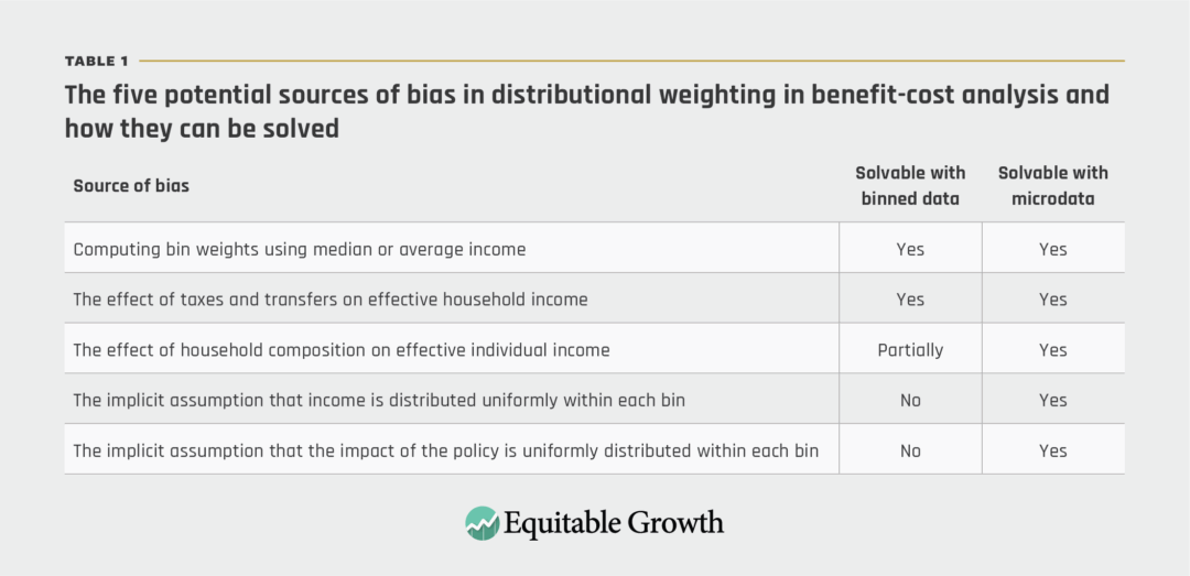
There are several limitations to this basic methodology. First, there are a number of biases that arise, which I address below and which my co-authors and I have developed ways to overcome. The five sources of bias break down into those that can be addressed using binned data and those that cannot and thus require a different approach. Second, the methodology requires assigning some proportion of unweighted impact to each income bin. The correct proportions may not be known and may require some arbitrary assumptions. And third, binned income data are often not available for the populations affected by a policy.

Most of these limitations cannot be addressed when using binned data, but all can be addressed by using microdata—datasets of information about large samples of individuals and/or households—using a methodology I present later in this report. But first, let’s examine these biases and see how some of them can be addressed by modifying the basic methodology.

Dealing with biases that arise in the basic benefit-cost methodology

There are five sources of bias that arise in the basic methodology described above. These biases have not been addressed in existing weighting applications. They are:

• The computation of bin weights using median or average income
• The unaccounted-for effect of taxes and transfers on effective household income
• The unaccounted-for effect of household composition on effective individual income
• The implicit assumption that income is distributed uniformly within each bin
• The implicit assumption that the impact of the policy is uniformly distributed within each bin

The first three of these biases can be addressed in the context of binned income data. The fourth and fifth cannot, but they can be addressed using microdata, as I explain later. In this section, I discuss each of these biases and how the first three can be addressed in binned data. (See Table 1.)

Table 1

Computing bin weights

Computing the bin weights as the weights at the midpoints of each bin biases the weights downward. The correct weight to use as the bin weight is the average weight across the bin.

The bias here arises because the weighting function is a hyperbola: It decreases fast as income increases at first, and then it decreases more slowly. Thus, for any given bin, the average weight for households with income below the midpoint will be above the weight at the midpoint by more than the average weight for households with income above the midpoint will be below the weight at the midpoint. Using the weight at the midpoint does not account for this, so it biases the weight for each bin downward.

An approximately unbiased bin weight can be achieved through a two-step method. First, we compute the weights at each of the endpoints of a bin and take the average of the two. This way of computing the weight is biased upward, but if you then take the average of this “midpoint of weights at the endpoints” and the “weight at the midpoint” from above, the upward and downward biases roughly cancel out.

Accounting for taxes and transfers

Weighting should be based on income that is actually available for consumption, after taxes and transfers are accounted for, to arrive at net income. The problem is, income data are usually reported pre-tax and pre-transfers, or gross income. Lower-income households typically receive more in transfers and pay less in taxes than higher-income households, so net income is higher than gross income for lower-income households and lower than gross income for higher-income households. This means that weights calculated using gross income are too high for low-income individuals and too low for higher-income individuals, introducing a bias in favor of low-income people.

My co-authors and I believe this undermines the legitimacy of weighting, making it important to do whatever is possible to account for taxes and transfers. Some data sources include income from public programs such as the Temporary Assistance for Needy Families program and Supplemental Security Income provided via the Social Security program. To account for the effect of taxes and of transfers in the form of tax credits such as the Child Tax Credit and Earned Income Tax Credit, my co-author, Dave Greenberg, and I used data from the National Bureau of Economic Research to compute a simple formula that transforms gross income into an approximation of net income.⁷ This formula doesn’t account for state and local taxes, but it helps to overcome the bias.

Accounting for household composition

Weighting should be conducted at the individual level, but income data are usually reported at the household level. This means that weighting does not account for the fact that the same household income represents lower effective individual-level income for larger households than for smaller households. Larger households also can take advantage of economies of scale in household consumption.

To overcome this bias, an adjustment can be made at the household level through what is called equivalization, or converting household income into an approximation of effective individual income. But this cannot be done with binned data—which would not matter if household sizes were the same at all levels of income, but because the average number of earners goes up with the size of households, lower-income households are, on average, smaller than higher-income households. As a result, household income overstates effective individual income, or equivalized income, more for higher-income households than for lower-income households, thus understating the weights on higher-income households more than it understates them for lower-income households.

Ignoring household composition once again biases distributionally weighted benefit-cost analysis in favor of low-income households. Dave Greenberg and I have used data from the U.S. Census Bureau’s American Community Survey to compute a simple formula that can be used to approximate the average effect of equivalization on the weights at the midpoints and end points of each income bin, thus addressing the bias.⁸

This approach still assumes that household composition is the same in the affected population as in the population as a whole. In fact, the size of households varies across populations. My calculations show, for example, that Americans identifying as Hispanic in American Community Survey data live in households that have, on average, 0.85 more members than those who identify as non-Hispanics. Similarly, some devout religious households, on average, may have larger households.

Adjusting for household size correctly among these populations would give them a lower equivalized household income and thus higher distributional weights. Not accounting for these differences in household size across groups therefore biases distributionally weighted benefit-cost analysis against groups with larger households. This bias can be addressed only crudely, and with strong simplifying assumptions, when using binned income data. Conversely, it can be straightforwardly addressed when using microdata that contains information on household composition, which allows for equivalization at the household level for each affected population.

Biases that cannot be addressed when using binned data

When using binned data, there is an implicit assumption that income, as well as the per-person impact of the policy being evaluated using benefit-cost analysis, are distributed uniformly within each bin. Both of these assumptions are likely to be violated in many cases, and both of them introduce bias.

If, for example, there are actually more people at the upper end of a bin than the lower end, or if individuals at the upper end of a bin experience a greater impact than individuals at the lower end of the bin, then the weighting methodology presented above will assign too little impact to the upper end of the bin, where the true weights are relatively low, and too much impact to the lower end of the bin, where the true weights are relatively high.

This would impart an upward bias to the bin weight. The bias would be downward if the number of people, or the per-person impact, are skewed toward the bottom of a bin. There is nothing that can be done about this when using binned data, but using microdata solves the problem automatically—an advantage that I detail in the next section of this report.

Solving problems and expanding the range of applications with microdata

Suppose you had microdata on the actual populations affected by a policy under review using benefit-cost analysis, including their incomes, their household compositions, and the unweighted cost or benefit each individual would experience as a result of the policy. All of the problems described above would go away.

Instead of worrying about bias in bin weights, you would compute weights for each individual. You could apply tax-and-transfer adjustments to each household and then equivalize household income based on the actual household composition of each household. As such, you could automatically address the possibility that household composition in an affected population might differ from the population as a whole.

What’s more, you would not have to make any assumptions about the distribution of income, or of per-person impact, within income bins, or the proportion of impact to assign to each bin. All methodological concerns and sources of bias would be addressed.

Needless to say, this is almost never the case because we typically do not have data on the exact population affected by the policy, or the unweighted cost or benefit to each individual. But something close can be achieved with the right methodology and some approximating assumptions.

In very simple terms, you need two things. First, you need microdata, and if you do not have microdata for the actual affected population, you only need a sample that can plausibly be treated as representative of the affected population. Second, in the highly likely scenario that the microdata you use do not include the actual per-person impact of the policy being assessed, you only need some individual-level proxy measure that can plausibly be treated as directly proportional to the actual per-person impact.

Next, I detail some examples of each of these two required things and then present some perhaps illuminating results.

Identifying the affected population in microdata

Sometimes microdata are available for the actual affected population of a given policy. Just one case in point: In a distributional weighting analysis I am currently doing for the Washington Center for Equitable Growth for a rule of the federal Administration for Children and Families that will affect Head Start early childhood education programs,⁹ I needed data on households with children in Head Start programs. Such data are publicly available in the National Survey of Early Childhood Education, conducted by the National Opinion Research Center at the University of Chicago.

Similarly, for a project on the effect of a proposed regulation governing talc-containing consumer products by the U.S. Food and Drug Administration,¹⁰ I needed data on consumers of a particular category of consumer products. I was able to obtain “homescan” data on all purchases made by a representative sample of households and identify the affected category of products, providing data on the actual consumers of the products. This was proprietary data, which are usually only made available for a price. My co-author was able to obtain it for free through his academic affiliation, but government agencies have invested in similar proprietary datasets.

In most of the work I have done, however, microdata are not available for the affected population. Here are some examples of how I have used existing datasets to create plausibly representative samples, what I call synthetic populations.

For the product safety regulation mentioned above, we needed data on the shareholders in publicly traded firms in the affected industry to compute the distributionally weighted cost of firms’ compliance with the regulation. Every 3 years, the Federal Reserve Board conducts the Survey of Consumer Finances, which includes information about ownership of corporate equities in a representative sample of the U.S. population. By making the assumption that the income distribution of shareholders in the affected industry was the same as in the general population of shareholders, we were able to use the Survey of Consumer Finances as a synthetic population that approximates the population of shareholders in the regulated industry.

For the Head Start rule mentioned above, I needed data on Head Start teachers, who will receive increases in monetary and nonmonetary compensation as a result of the rule. The National Survey of Early Childhood Education has information on Head Start teachers, but household income is top-coded to protect confidentiality at $60,000, which is not very helpful for distributional weighting.

By computing the joint distribution of five key observable characteristics of Head Start teachers in the National Survey of Early Childhood Education data, I was able to construct a synthetic population in American Community Survey data by identifying preschool teachers by their occupational code and randomly selecting a sample with the same joint distribution of those five characteristics. The five characteristics were marital status, educational attainment (below or above the associate’s degree level), White or non-White, age (in three categories), and whether the teachers’ households received some kind of government assistance.

I chose those five variables because they showed the most difference between Head Start and non-Head Start teachers in the NSECE data, giving them maximum power to identify hypothetical Head Start teachers in the ACS data. They are also correlated with income, such that a population that is representative on these five characteristics is likely to be representative on income. I could have chosen more variables or more categories of each variable, but the number of teachers in each subcategory in the NSECE data would have gotten too small to be statistically significant.

In another analysis I am currently doing for the Washington Center for Equitable Growth—on a proposed workplace-safety rule by the federal Occupational Safety and Health Administration that would reduce heat-related injuries and illnesses¹¹—I needed data on the population of workers who would be affected by the rule. The U.S. Bureau of Labor Statistics maintains the Survey of Occupational Injuries and Illnesses, which contains data on each individual who experiences heat-related injury and illness.

These data could potentially be used to conduct distributional weighting on the population affected by the rule. Obtaining data from this dataset, however, requires a special query request, and there is a delay of several months on responses to such requests, which could be prohibitive to timely analysis. And the data do not include household income or household composition, so would need to be combined with some other dataset.

Instead, I again turned to the American Community Survey and identified individuals working in industries and occupations—and living in locations—that involve significant workplace heat exposure. I categorized occupations by heat exposure using data from the Occupational Information Network, or O*NET, which is maintained by the Bureau of Labor Statistics. I obtained data on ambient heat index by state from the National Weather Service. I identified industries with particularly high heat exposure using data from the Notice of Proposed Rule Making for the rule.¹² All of these sources are publicly available, though downloading the data from the National Weather Service required a Python script, which I developed in about 2 hours using generative artificial intelligence. This provided me with a synthetic population that is arguably approximately representative of workers affected by the rule.

Finding proxy measures for the per-person impact of the policy

Obviously, in addition to information about income and household composition, you also need some kind of information about the impact that accrues to each individual in the synthetic population. Fortunately, it is not necessary to know the actual dollar value for each household, provided you have information about some proxy measure that can be assumed to be directly proportional to the dollar value.

This is because, in the methodology my co-authors and I have developed, we are not actually computing distributionally weighted cost or benefit directly.¹³ Instead, we are computing the ratio of distributionally weighted cost or benefit to unweighted cost or benefit, which can be thought of as the distributionally weighted cost or benefit as a proportion of unweighted cost or benefit. We call this number the “population weight” for a given cost or benefit to a given population.

If you know this population weight, and you know the unweighted cost or benefit to the population, then you can simply multiply these together to get an estimate of the distributionally weighted cost or benefit. If the population weight on the cost of a product-safety regulation on consumers (through price increases) is 1.5, for example, it means that the distributionally weighted cost is 1.5 times the unweighted cost.

The unweighted cost will typically have been computed using industrywide data on costs that do not take into account the distribution of the burden borne by different stakeholders in the firms that are being regulated. To compute population weights, it is not necessary to know the actual dollar value of the cost or benefit experienced by each individual. It is only necessary to be able to identify or compute some proxy measure that is proportional to the dollar value of the impact.

To compute the population weight on the cost of regulatory compliance with the talc rule borne by consumers, for example, we found data on the quantity of the regulated products consumed by each household in a dataset of consumer purchases and assumed that the cost would be passed on to consumers in proportion to the quantity of the products consumed. This is a plausible assumption, given that the cost comes in the form of price increases.

So, the true dollar value is the quantity consumed multiplied by some unknown number that represents the dollar cost per ounce of product. Having identified this proxy measure, we multiply it by the distributional weight for each household to get the distributionally weighted proxy. Then, we compute the sum of the distributionally weighted proxy across households and the sum of the unweighted proxy, and take the ratio of the two. This ratio is the same as the ratio of distributionally weighted cost-to-unweighted cost, because the unknown number that represents the dollar cost per ounce of product appears in both sums and thus cancels out of the ratio.¹⁴

Below are some examples of proxy measures I have developed in the work I am currently doing, funded by the Washington Center for Equitable Growth.

To compute the population weight for the benefit of the Head Start rule to households with children in Head Start programs, I assumed that the benefit to each household was directly proportional to the number of Head Start children in the household, which is available in the National Survey of Early Childhood Education. Again, to compute the population weight, I didn’t need to know the actual benefit of the rule to individual children. I only needed to assume that it is the same across children, which is the kind of approximating assumption typically made throughout benefit-cost analyses.

To compute the population weight for the benefits of the heat rule for workers, I created a heat-exposure index that is a function of days of exposure to hot environments by occupation from O*NET data, the heat exposure level of industries from the Notice of Proposed Rule Making for the regulation, the average hourly ambient heat index by state from National Weather Service data, and the number of hours worked per worker from the American Community Service data. A number of assumptions must be made to be able to treat this index as directly proportional to the dollar value of reduced heat-related injury and illness. But those assumptions are on par with the kinds of assumptions that are routinely made in many unweighted benefit-cost analyses.

What is the same across all of these examples is that binned income and impact data were not available. By using synthetic populations and proxy measures of impact, both powered by microdata, I was able to significantly expand the range of applications of distributional weighting. I have used the same methodology to compute population weights for the cost of regulatory compliance to shareholders, participants in defined-benefit retirement plans, and stakeholders in nonprofits that invest in equities. I also have used this methodology to compute population weights on the burden of the federal tax system on the U.S. population and the benefits of the Head Start rule to noneducational Head Start staff.¹⁵

Some interesting results on population weights

The population weights I have computed have been informative in sometimes interesting or even surprising ways. I have heard people claim, for example, that if the benefits of a policy accrue to the same population as the costs, then distributional weighting is redundant. But this assumes that the distribution of benefits across the affected population is the same as the distribution of costs.

Yet in my analysis of the consumers of the products regulated under the FDA rule mentioned above, I found that this was not the case. Instead, I found that the distribution of cost was skewed more heavily toward the lower end of the income distribution among consumers than the distribution of benefit. In other words, the same people experienced both cost and benefit, but the households that experienced the highest benefit were not the same as the households that experienced the highest cost. The former, on average, were higher income than the latter. (See Figure 1.)

Figure 1

The population weight for consumer benefits of the FDA talc rule, shown in Panel 1 of Figure 1, was 1.397, while for consumer costs, the population weight was 1.957—a difference of 40 percent. What that means is that the true increase in welfare (the distributionally weighted benefit) was 1.397 times greater than the unweighted benefit, and the true decrease in welfare (the distributionally weighted cost) was 1.957 times greater than the unweighted cost.

A benefit-cost analysis that found that the unweighted benefit to consumers was greater than the unweighted cost might be reversed by distributional weighting because the unweighted cost would be increased by distributional weighting more than the unweighted benefit. Suppose, for example, that the unweighted benefit was $10 million and the unweighted cost was $9 million. The distributionally weighted benefit (meaning the true increase in welfare) would be $13.97 million and the distributionally weighted cost would be $17.61 million.

Because the costs hit lower in the income distribution than the benefits, and because the value of a dollar goes up as income goes down, the unweighted measure gave the wrong answer. The actual welfare impact of the $9 million unweighted cost, because it disproportionately hit people for whom the value of a dollar was particularly high, was significantly greater than the welfare impact of the $10 million unweighted benefit, which disproportionately hit people for whom the value of a dollar was not quite as high.

Another interesting finding relates to who bears how much of the costs of policies. I believe there is a general assumption that the part of the cost of regulatory compliance borne by publicly traded firms falls ultimately on the quite wealthy shareholders in those firms and that, as a result, distributional weighting will significantly deflate those costs. In my analysis of the FDA rule, however, I computed a population weight on the cost of compliance to firms of 1.032, pretty much equal to the weight at median income. This is because almost 40 percent of U.S. equities are held by nonprofit organizations, and the cost of compliance borne by those investors ultimately passes through to those who receive the benefits of the activities of those nonprofit organizations.

Even under the arguably conservative assumption that those benefits are evenly distributed across the general population, the distribution of income in the United States is so heavily right-skewed (meaning that there are a large number of quite low-income households and a smaller number of very wealthy households) that the population weight on the cost of compliance to nonprofit shareholders was 2.044—enough to balance out the much smaller population weight of 0.447 on household shareholders.¹⁶ (Note that to compute the weighted cost of compliance, it was necessary to also compute the population weight on the cost borne by participants in defined-benefit pension plans—the other main category of institutional investors—and then compute the proportionally weighted average of all of the cost-related population weights.)

I was similarly quite surprised by the results of my analysis of the Head Start rule mentioned above. It turns out that while Head Start teachers earn only a little from their own labor, they disproportionately live in households that include much-higher-earning members. So, despite the presence of quite a lot of unmarried individuals living alone among Head Start teachers, the population weight of Head Start teachers was 0.713, a fair bit below 1, the weight at the median. I had expected it to be quite a bit above 1 because I had a mistaken belief about the financial circumstances of Head Start teachers.

Still, this population weight on Head Start teachers is greater than the population weight I computed for the taxpayers who bear the cost of the rule, which was 0.509. The unweighted benefit to teachers is $1.18 billion, while the unweighted cost to taxpayers was $1.89 billion, a benefit-cost ratio of 0.624, making the rule seem like a poor investment. When distributional weights are applied, the benefit (in welfare terms) is deflated to $980 million, but the cost to taxpayers (again, in welfare terms) is deflated more, to $960 million, a benefit-cost ratio of 1.015. The rule breaks even.

Now, although there is some controversy over whether teacher pay affects the outcomes of the children participating in Head Start programs, and although the Administration for Children and Families did not include the benefit to the children enrolled Head Start in its benefit-cost analysis, the population weight for households with children in Head Start was greater than 4. So, it would not take much benefit to households with children in Head Start to increase the weighted benefit-cost ratio significantly.

Finally, the results for the OSHA heat rule are interesting. The unweighted benefit (from reduced heat-related fatality, injury, and illness) and cost (of the steps necessary for firms to comply with the rule), calculated by the agency in their preliminary regulatory impact analysis, were $9.2 billion and $7.8 billion, respectively. The unweighted net benefit was thus $1.4 billion, and the benefit-cost ratio was 1.18, which is only marginally above the threshold of 1, above which the rule passes the benefit-cost test.

My own intuition, before conducting the analysis, was that the weight on benefits to workers would be fairly high, and the weight on cost of compliance to firms would be fairly low, leading the weighted benefit-cost ratio—the return on investment in welfare terms—to be considerable higher. This is not what I found in my analysis. The population weight on the benefit to workers was 1.019. Workers in occupations, industries, and states with high heat exposure are not predominantly in very low-income positions or very low-income households. The weight on the cost borne by consumers (in the form of price increases) and owners of firms (both private and publicly traded) were 1.047 and 0.852, respectively.

A review of available evidence on elasticities of supply and demand in different sectors of the economy suggests that consumers will bear something like 44 percent of the heat rule burden. Using that proportion to calculate a weighted average of the population weights on cost to owners of firms and cost to consumers produces a weight that can be applied to the total cost of compliance. That weight is 0.938. The stakeholders of the firms that bear the cost of compliance are not, on balance, particularly high income. Thus, the weighted benefit was $9.4 billion and the weighted cost was $7.3 billion, for a benefit-cost ratio of 1.29, not much above the unweighted benefit-cost ratio.

Feasibility of using microdata

The work I have done using synthetic populations and proxy impact measures requires some creativity and some proficiency with statistical software such as Microsoft Excel and Stata. As an economist, I am reasonably well-versed in each of those pieces of software and have some experience with making the kinds of assumptions described above. But my expertise is not greater than what I have encountered at numerous regulatory agencies.

As I explained in the opening section of this report, my goal is for distributional weighting to be practical for use by smaller agencies and nonprofit organizations that may be less “teched up.” One lesson I have learned is that I can save myself enormous amounts of time by using generative AI to help figure out analytical puzzles, and even to write code for me.

Downloading and concatenating several thousand National Weather Service files, which did not contain a needed state identifier, required a Python script. I do not know Python and did not have time to learn it. Instead, I used ChatGPT to write a Python script to do the downloading and concatenation for me. It took me several hours of going back and forth with the bot to debug the script and get it to work, but this was orders of magnitude less time consuming than downloading the files manually or learning Python—and a lot cheaper than paying a consultant.

Over the past few years, largely in response to the Biden administration’s revisions of the Circular A-4, a number of academics have expressed doubts, concerns, and outright rejection of distributional weighting. An often heard but seldom justified claim is that the data requirements of distributional weighting are likely to be insuperable in many or most cases. Several academic articles have made this claim.¹⁷ In a letter to the Biden administration’s director of the Office of Information and Regulatory Affairs signed by 15 former presidents of the Society for Benefit Cost Analysis and former editors of the Journal of Benefit Cost Analysis, the concern about practicability is raised, and the authors conclude: “In most cases, agencies do not have the experience or tools to do this.”¹⁸

Having worked for a year at the Food and Drug Administration, and having collaborated with FDA economists on distributional weighting, I can say affirmatively that with appropriate guidance and methodological tools, there is certainly a future in which agencies will have the experience and tools to do distributional weighting. The work I did, for example, with generative AI to build the Python codes that I needed to complete my distributional weighting will only become easier in the years ahead—and so also will others’ ability to conduct distributional weighting.

Next steps

The worst-case scenario for distributional weighting is for every analyst to have to reinvent the wheel, starting from the terse and incomplete guidance provided in government guidance documents, which I foresee will result in many—perhaps most—analysts and organizations concluding that weighting is infeasible. I also foresee that without guidance, whatever distributional weighting is done will be conducted with overly simplistic methodologies that create potentially significant biases, when solutions to overcome those biases are readily available and easy to implement.

As I mentioned above, my ultimate goal is to create something like an instruction manual, which will take the form of a free pdf and/or a website. It will lay out all of the steps referenced above—including Stata, R, and Python code for steps such as conducting equivalization—and it will go into detail on how to implement the methodologies that my co-authors and I have developed.

One possibility is that future administrations will return to distributional weighting. If so, there will be work to do in supporting agencies in conducting distributional weighting. The analysis we published in the Federal Register stands as proof that the work can be done. Building relationships with agency analysts and personnel at the White House Office of Management and Budget will be part of the work. Opportunities to provide hands-on guidance could advance the work.

In the meantime, there are other entities that conduct benefit-cost analysis that may be interested (or may become interested) in conducting distributional weighting. Some state government agencies and nonprofit organizations, as well as agencies in other countries or regions such as the European Union, may fall into this category. My intention is to promote the methodologies of distributional weighting wherever I may find a receptive welcome, and to lay the groundwork for analysts to implement this important and ethically responsible set of tools.

About the author

Dan Acland is an associate professor of research at the Goldman School of Public Policy at the University of California, Berkeley. His research revolves around benefit-cost analysis and is currently focused primarily on issues of equity in benefit-cost analysis, including the conceptual and practical issues that arise in distributional weighting to address bias against low-income people. His work on distributional weighting has been published in the Journal of Benefit Cost Analysis, the Journal of Policy Analysis and Management, and the Annals of Public and Cooperative Economics.

Acknowledgements

The author would like to thank David S. Mitchell, Raj Nayak, and Equitable Growth’s editorial team for invaluable comments on earlier drafts. Any and all errors are the author’s own.